Project 2 - Rankine cycle Simulator
Program:
%% Rankine Cycle Simulator
%%
% Program to find the thermal efficiency, back work ratio and the state
% points of the rankine cycle

clear all
close all
clc

% inputs for calculating Rankine cycle
p1 = input('Enter the inlet pressure of turbine:   ')
p2 = input('Enter the outlet pressure from turbine:  ')
t1 = input('Enter the steam inlet temperature:   ')

% pressure of state points
p4 = p1;
p3 = p2;

% Cycle information
fprintf('Process 1-2 : Isentropic expansion process (Turbine)\n')
fprintf('Process 2-3 : isobaric heat rejection process (Condensor)\n')
fprintf('Process 3-4 : Isentropic compression process (Pump)\n')
fprintf('Process 4-1 : Isobaric heat addition process (Boiler)\n')


%calculating the dryness fraction of state points

s1 = XSteam('s_pT',p1,t1); % state point 1

s2 = s1; % state point 2
sf2 = XSteam('sL_p',p2);
sg2 = XSteam('sV_p',p2);
sfg2 = sg2 - sf2;
x2 = (s1 - sf2)/sfg2;


if (x2 > 1)
    t2 = XSteam('T_ps',p2,s2);
    t_2 = XSteam('Tsat_p',p2);
    t3 = t_2;
    Td = linspace(t2,t_2,50);
    s_2 = XSteam('sV_T',t_2);
    s3 = XSteam('sL_T',t3);
    s4 = s3;
else
    t2 = XSteam('Tsat_p',p2);
    t_2 = t2;
    t3 = t2;
    s3 = sf2; % State pont 3
    s4 = s3; % state point 4


end

%calculating the enthalpy of state points

h1 = XSteam('h_pT',p1,t1); % state point 1

hf2 = XSteam('hL_p',p2); % state point 2
hg2 = XSteam('hV_p',p2);
hfg2 = hg2 - hf2;
h2 = hf2 + x2*hfg2;

h3 = hf2; % state point 3

v3 = XSteam('vL_p',p3); %specific volume

h4 = v3*(p1-p2)*100  + h3; % state point 4

cp = XSteam('Cp_ps',p3,s3);
cv = XSteam('Cv_ps',p3,s3);
k = 1 - (cv/cp);
t4 = t3*((p4/p3)^k);

t5 = XSteam('Tsat_p',p1);
t6 = t5;

s5 = XSteam('sL_T',t5);
s6 = XSteam('sV_T',t6);


% Turbine work
Wd_tb = h1 - h2;

% Pump work
Wd_pm = h4 - h3;

% Net work, Back work ratio and thermal efficiency of Rankine cycle
W_net = Wd_tb - Wd_pm;
bwr = (h1 - h4)/(h2 - h3);
efficiency = W_net/(h1-h4);
efficiency = efficiency*100;
% state point 1 parameters
fprintf('\n\t\t\tResults\n')
fprintf('\nState point-1')
fprintf('\nP1 = %f',p1)
fprintf('\nT1 = %f',t1)
fprintf('\nS1 = %f',s1)
fprintf('\nH1 = %f',h1)


% state point 2 parameters

fprintf('\n\nState point-2')
fprintf('\nP2 = %f',p2)
fprintf('\nT2 = %f',t2)
fprintf('\nS2 = %f',s2)
fprintf('\nH2 = %f',h2)
fprintf('\nX = %f',x2)


% state point 3 parameters

fprintf('\n\nState point-3')
fprintf('\nP3 = %f',p3)
fprintf('\nT3 = %f',t3)
fprintf('\nS3 = %f',s3)
fprintf('\nH3 = %f',h3)


% state point 4 parameters

fprintf('\n\nState point-4')
fprintf('\nP4 = %f',p4)
fprintf('\nT4 = %f',t4)
fprintf('\nS4 = %f',s4)
fprintf('\nH4 = %f',h4)

% Performance parameters of Rankine cycle

fprintf('\n\n Performance of Rankine cycle')
fprintf('\nTurbine work = %f',Wd_tb)
fprintf('\nPump work = %f',Wd_pm)
fprintf('\nBack Work ration = %f',bwr)
fprintf('\nThermal efficiency = %f',efficiency)

%plotting of the graph

% Data - boiler sensible heat addition at superheated condition
T = linspace(t6,t1,500);
for i = 1:length(T)
    S(i) = XSteam('s_pT',p1,T(i));
    H(i) = XSteam('h_pT',p1,T(i));
end

% Data - saturation temperature curve
maxt = linspace(1,t1,500);
for j = 1:length(maxt)
    satlS(j) = XSteam('sL_T',maxt(j));
    satvS(j) = XSteam('sV_T',maxt(j));
    satlH(j) = XSteam('hL_T',maxt(j));
    satvH(j) = XSteam('hV_T',maxt(j));
end
%%
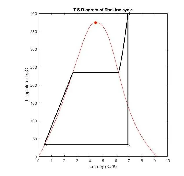
%% T-S Diagram for Rankine cycle
subplot(1,2,1)
% plot - saturation curves
plot(satlS,maxt,'color','r')% saturation liquid temperatures
hold on
plot(satvS,maxt,'color','r')% saturation vapour temperatures
plot(4.4230,373.6,'o','MarkerFaceColor','r','MarkerSize',7) % critical temperature

%plot - Curve for points t5 and t6
line([s5 s6],[t5 t6],'Color','k','lineWidth',2)
%plot - Curve for points t6 and t1
plot(S,T,'Color','k','lineWidth',2)
%plot - Curve for points t1 and t2
line([s1 s2],[t1 t2],'Color','k','lineWidth',2)

if (x2 > 1)
    % Data - constant pressure curve at boiler inlet if present
    for i = 1:length(Td)
    Sd(i) = XSteam('s_pT',p2,Td(i));
    Hd(i) = XSteam('h_pT',p2,Td(i));
    end

%plot - Curve for points t2 and t_2 (if present)
plot(Sd,Td,'color','k','lineWidth',2)
% plot - line for t_2 and t3 (if present)
line([s_2 s3],[t_2 t3],'Color','k','lineWidth',2)
else
    line([s2 s3],[t2 t3],'color','k','lineWidth',2)
end

%plot - Curve for points t3 and t4
line([s3 s4],[t3 t4],'Color','k','lineWidth',2)

% plot - Constant pressure heat addition curve till saturation liquid line
line([s4 s5],[t4 t5],'Color','k','lineWidth',2)

% labelling of graph
title('T-S Diagram of Rankine cycle')
xlabel('Entropy (KJ/K)')
ylabel('Temprature degC')

% Marking the state points
text(s1,t1,"1");
text(s2,t2,"2");

if (x2 > 1)
    text(s_2,t_2,"2'");
end
text(s3,t3,"3");
text(s4,t4,"4");


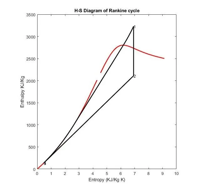
%% H-S diagram for rankine cycle
subplot(1,2,2)
% plot for saturation curves of liquid and vapuor
plot(satlS,satlH,'color','r','lineWidth',2)
hold on
plot(satvS,satvH,'color','r','lineWidth',2)

% plot - isentropic expansion line
line([s1 s2],[h1 h2],'color','k','lineWidth',2)


if (x2 > 1)

    h_2 = XSteam('h_ps',p2,s_2);
    %plot - constant pressure heat addition ,if outlet steam is superheatedcond.
    plot(Sd,Hd,'color','k','lineWidth',2)

    % Data - constant pressure heat rejection curve enthalpy values
    entrpy = linspace(s_2,s3,100);
    for k = 1:length(entrpy);
        enthlpy(k) = XSteam('h_ps',p2,entrpy(k));
    end

    % Plot - constant pressure heat rejection curve
    plot(entrpy,enthlpy,'color','k','lineWidth',2)
else

    % Data - constant pressure heat rejection curve enthalpy values if
    % steam is wet or dry saturated vapour
    entrpy = linspace(s2,s3,100);
    for k = 1:length(entrpy);
        enthlpy(k) = XSteam('h_ps',p2,entrpy(k));
    end

     % Plot - constant pressure heat rejection curve
    plot(entrpy,enthlpy,'color','k','lineWidth',2)
end

%plot - Isentropic compression line
line([s3 s4],[h3 h4],'color','k','lineWidth',2)

% data - Constant pressure heat addition curve enthalpy values
entrpy1 = linspace(s4,s1,100);
for l = 1:length(entrpy1)
    enthlpy1(l) = XSteam('h_ps',p1,entrpy1(l));
end

% plot - Constant pressure heat addition curve
plot(entrpy1,enthlpy1,'color','k','lineWidth',2)

% labelling of graph
title('H-S Diagram of Rankine cycle')
xlabel('Entropy (KJ/Kg K)')
ylabel('Enthalpy KJ/Kg')

% Marking the state points
text(s1,h1,"1");
text(s2,h2,"2");

if (x2 > 1)
    text(s_2,h_2,"2'");
end
text(s3,h3,"3");
text(s4,h4,"4");

%%
Steps:
- Initially, it takes in values for the inlet, outlet conditions of turbine and boiler temperature
- Then it calculates the entropy for second state point as expansion in turbine is isentropic. values for entropies and other data in the code is exported fromthe XSteam.m file given.
- using the obtained data entropy at third state point is known with which entropy at boiler inlet is also obtained as pump in an isentropic process
- Similarly values for enthalpy is also found out.
- using the appropriate formulas and the data generated the performance parameters of the rankine cycle is found out.
- The required data as asked is printed as output.
- For plotting of T-S diagram : isentropic process and constant pressure heat addition and rejection at latent heat temperature follow a straight line. So, can be plotted with two end points
- For constant pressure heat addition and rejection at sensible heat temperatures it follows the constant pressure line hence data is to be generated at each point. This is done by making use of a for loop
- Finally if the dryness fraction is grater than one at turbine outlet condition then heat rejection in condensor will initially follow the constant pressure curve until it reaches the saturation vapour temperature. if less than one the steam is wet in condition.
Result:
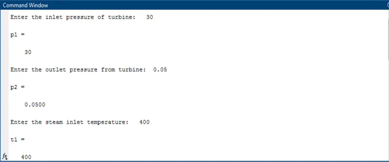

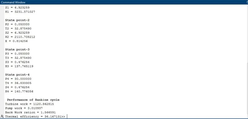
Plot:
T-S diagram and H-S diagram:
Coclusion:
A code to simulate the Rankine cycle is done with calculation for performance parameters along with plots for T-S and H-S diagram.
References: