Project 2 - Rankine cycle Simulator
Rankine cycle simulator
close all
clear all
clc
% print process discription
fprintf('1-2 Isobaric heat transfer/n')
fprintf('2-3 Isentropic heat Expansion/n')
fprintf('3-4 Isobaric heat rejection/n')
fprintf('4-1 Isentropic heat compression/n')
% Enter inputs
p1 = 30;
T1 = 400;
p2 = 0.5;
% state point 1
h1 = Xsteam('h_pT',30,400);
s1 = Xsteam('s_pt',p1,T1);
% state point 2
s2 =s1;
sf2 = Xsteam('sL_p',p2);
sg2 = Xsteam('sV_p',p2);
hf2 = Xsteam('hL_p',p2);
hg2 = Xsteam('hV_p',p2);
s2 = sg2; % x2 = (s2-sf2)/(sg2-sf2);
h2 = hg2; % hf2 + (x2*(hg2-hf2));
T2 = Xsteam('T_hs',h2,s2);
% state point 3
T3 = T2;
p3 = p2;
s3 = Xsteam('sL_t',T3);
h3 = Xsteam('hL_T',T3);
v3 = Xsteam('vl_p',p2);
% state point 4
p4 = p1;
s4 = s3
cp4 = Xsteam('Cp_ps',p4,s4);
cv4 = Xsteam('Cv_ps',p4,s4);
gamma = cp4/cv4;
r = (gamma-1)/gamma;
T4 = T3*(p4/p3)^r;
% calculate other output values
wt = h1-h2; % Turbine work
wp = v3*(p1-p2)*100; % pump work
h4 = wp+h3;
w_net = wt - wp; % net work unit in kj/kg
Qs = h1 - h4; % heat supplied
N_per = (w_net/Qs)*100; % Efficiency
steam_rate = 3600/(wt-wp); % steam rate per second
% All point which help in plotting.
T5 = Xsteam('Tsat_p',p1);
T6 = T5;
s5 = Xsteam('sL_p',p1);
s6 = Xsteam('sV_p',p1);
h5 = Xsteam('hL_p',p1);
h6 = Xsteam('hV_p',p1);
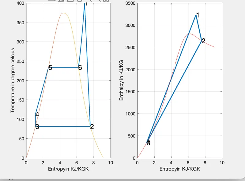
% plot T-s diagram
subplot(1,2,1);
T_Rankine = linspace(T5,400,500);
for i = 1:length(T_Rankine);
s_rankine(i) = Xsteam('s_pT',p1,T_Rankine(i));
end
plot([s1 s2 s3 s4 s5 s6 s_rankine],[T1 T2 T3 T4 T5 T6 T_Rankine],'linewidth',1.5);
hold on
grid on
T_curve = linspace(1,400,5000);
for i= 1:length(T_curve);
s_l(i) = Xsteam('sL_T',T_curve(i));
s_v(i) = Xsteam('sV_T',T_curve(i));
h_l(i) = Xsteam('hL_T',T_curve(i));
h_v(i) = Xsteam('hV_t',T_curve(i));
end
plot(s_l,T_curve);
plot(s_v,T_curve);
text(s1,T1,'1','Fontsize',15);
text(s2,T2,'2','Fontsize',15);
text(s3,T3,'3','Fontsize',15);
text(s4,T4,'4','Fontsize',15);
text(s5,T5,'5','Fontsize',15);
text(s6,T6,'6','Fontsize',15);
xlabel('Entropyin KJ/KGK')
ylabel('Temprature in degree celcius')
% plot H-S Diagram
subplot(1,2,2)
plot([s1 s2 s3 s4 s1],[h1 h2 h3 h4 h1],'linewidth',2)
hold on
grid on
plot(s_v,h_v,'color','r');
plot(s_l,h_l,'color','r');
text(s1,h1,'1','FontSize',15);
text(s2,h2,'2','FontSize',15);
text(s3,h3,'3','Fontsize',15);
text(s4,h4,'4','Fontsize',15);
xlabel('Entropyin KJ/KGK');
ylabel('Enthalpy in KJ/KG');
Basic Rankine Cycle
OUTPUT VALUES
State point :1
P1 : 30 bar
T1 : 400 Degree Celicious
H1 : 3.2316e+03 KJ/KG
S1 : 6.9233 kJ/KGK
State point :2
P2 : 0.5 Bar
T2 : 81.3161 Degree Celsius
H2 : 2.6452e+03 KJ/KG
S2 : 7.5930 KJ/KGK
State point :3
P3 : 0.5 Bar
T3 : 81.3161 Degree Celsius
H3 : 340.4733 KJ/KG
S3 : 1.0910 KJ/KGK
State point :4
P4 : 30 Bar
T4 : 112.5850 Degree Celcious
H4 : 343.5116 KJ/KG
S4 : 1.0910 KJ/KGK
WT : 586.3578 KJ/KG
WP : 3.0382 KJ/KG
WNET : 583.3195 KJ/KG