Project 2 - Rankine cycle Simulator
PROJECT 2 - RANKINE CYCLE SIMULATOR
Aim :-
- Create a Rankine Cycle Simulator using MATLAB.
Objective :-
- Calculate the state points of the Rankine Cycle based on user inputs.
- Plot H-S & T-S diagram.
- To get all output in Command window.
Theory :-
Rankine Cycle :-
Two primary classes of thermodynamic cycles are power cycles and heat pump cycles. Power cycles are cycles which convert some heat input into a mechanical work output, while heat pump cycles transfer heat from low to high temperatures by using mechanical work as the input.
Rankine Cycle Process :-
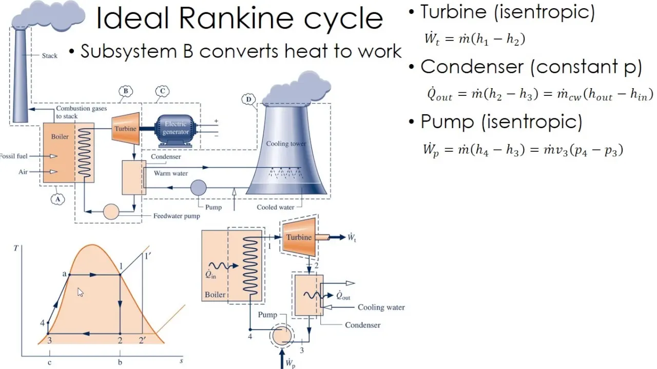
1)Process 1-2: Isentropic Expansion in Turbine
The dry saturated vapour expands through a turbine, generating power.
2)Process 2-3 : Constant pressure heat rejection in condensor
The wet vapour then enters a condenser, where it is condensed at a constant pressure to become a saturated liquid. Process 4-1 is constant pressure heat rejection in condenser.
3)Process 3-4 : Isentropic compression in feed pump
The working fluid is pumped from low to high pressure. As the fluid is a liquid at this stage, the pump requires little input energy.
4)Process 4-1 : Constant pressure heat addation in boiler
The high-pressure liquid enters a boiler, where it is heated at constant pressure by an external heat source to become a dry saturated vapour.
Required Inputs:
Turbine Inlet temperature = 400° C.
Turbine Inlet Pressure = 30 bars.
Turbine Outlet Pressure = 0.05 bars = Condenser Inlet Pressure.
Equations used :-
Qin :- h1-h4
wt :- h1-h2
Qout :- h2-h3
Wp :- h4-h3
Thermal Efficiency :- (Wnet/Qin)*100
Matlab Code and step explaination :-
Step No. 1 :- To print all process description in cmd window we used 'fprintf' cmd
clear all
close all
clc

% print process description

fprintf('1-2 Isentropic Expansion in the turbine\n');

fprintf(['2-3 Constant pressure heat rejection at condenserrankine Cycle simulator\n']);

fprintf('3-4 Isentropic compression by feed pump\n');

fprintf('4-1 constant pressure heat addation in boiler\n');
Step No.2 :- TO get user input like pressure at turbine inlet, inlet temp. of turbine & outlet pressure of turbine
% Input

p1=input('Entre the vlaue of pressure at turbine inlet(in bar):\n');

T1=input('Enter the value of temperature at turbine inlet(in ^°C):\n');

p2=input('Enter the value of pressure at condensor inlet(in bar):\n');
Step No. 3 :- Now we have to calculate state points values at state 1 to 4 for enthalpy and entropy at various temp. from XSteam file.
%calculating state points

% State point-1

h1 = XSteam('h_pT',p1,T1) % getting the value of enthalpy at p1 & T1

s1 = XSteam('s_pT',p1,T1) % getting the value of entropy at p1 & T1

% State point-2

s2 = s1;

sf2 =  XSteam('sL_p',p2);

sg2 = XSteam('sV_p',p2);

x2 = (s2-sf2)/(sg2-sf2);

hf2 = XSteam('hL_p',p2);

hg2 = XSteam('hV_p',p2);

h2 = hf2+(x2*(hg2-hf2));

% State Point-3

p3 = p2;

s3 = XSteam('sL_P',p3);

h3 = XSteam('hL_P',p3);

% State Point-4

s4 = s3;

p4 = p1;
Step No. 4 :- Now we to calculate the work done turbine, work supply to feed pump,net work,heat add in system, heat out of system,
Thermal efficiency, and Sep. steam consumption.
% Calculating work done by turbine

wt = h1-h2

% Work done to run the pump

v3 = XSteam('vL_P',p3);
wp = v3*(p4-p3)*100
h4 = h3+wp;

% Net work

wnet = wt-wp

% heat add into the cycle

Qin = h1-h4;

% heat out of the system

Qout = h2-h3

% Thermal Efficiency

eff = (wnet/Qin)*100

% Calculating Sp.Steam comsumption

SSC = (3600/wnet)
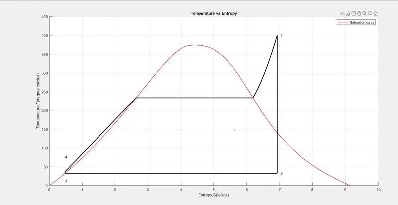
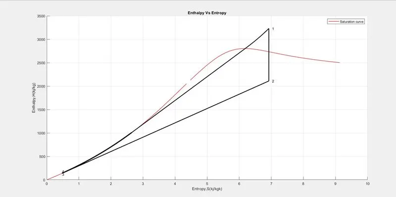
Step No. 5 :- By using for loop and plot cmd we plot T-S and H-S plot
% calculating Temp at state point 2,3,4

T3 = XSteam('Tsat_P',p3);

T2 = T3;

cp4 = XSteam('cp_ps',p4,s4);

cv4 = XSteam('cv_ps',p4,s4);

k = cp4/cv4;

T4 = T3/((p3/p4)^((k-1)/k));

% Calculating Temp, enthalpy,at staureated vapour and liquid

T6 = XSteam('Tsat_P',p1);

s5 = XSteam('sL_P',p1)

s6 = XSteam('sV_p',p1);

h5 = XSteam('hL_p',p1);

h6 = XSteam('hV_p',p1);

T5 = T6;

% plotting the saturation curve

T = linspace(1,375,1000);

for i=1:length(T)
    sf(i) = XSteam ('sL_T',T(i));
    sg(i) = XSteam ('sV_T',T(i));
    hf(i) = XSteam ('hL_T',T(i));
    hg(i) = XSteam ('hV_T',T(i));

end

% plotting T-S dig.

figure(1)
hold on

plot(sf,T,'Color','r','LineWidth',1)

plot(sg,T,'Color','r','LineWidth',1)

plot([s1 s2],[T1 T2],'k','LineWidth',2)

plot([s2 s3],[T2 T3],'k','LineWidth',2)

plot([s3 s4],[T3 T4],'k','LineWidth',2)

plot([s4 s5],[T4 T5],'k','LineWidth',2)

plot([s5 s6],[T5 T6],'k','LineWidth',2)

sc1 = linspace(s6,s1,1000);

for l=1:length(sc1)
   Tc1(l)=XSteam('T_PS',p1,sc1(l));
end

plot(sc1,Tc1,'k','LineWidth',2)

text(s1+0.1,T1,'1')
text(s2+0.1,T2,'2')
text(s3,T3-20,'3')
text(s4,T4+40,'4')

title('Temperature vs Entropy')
grid on
xlabel('Entropy,S(kj/kgk)')
ylabel('Temperature,T(degree celcius)')
legend('Saturation curve')


% plotting H-S diagram
figure(2)
hold on

plot(sf,hf,'Color','r','LineWidth',1)
plot(sg,hg,'Color','r','LineWidth',1)


plot([s1 s2],[h1 h2],'k','LineWidth',2)
plot([s2 s3],[h2 h3],'k','LineWidth',2)
plot([s3 s4],[h3 h4],'k','LineWidth',2)

hc=linspace(h4,h5,100);

for k=1:length(hc)
    sch(k)=XSteam('s_Ph',p1,hc(k));
end

plot(sch,hc,'k','LineWidth',3)
plot([s5 s6],[h5 h6],'k','LineWidth',2)

for m=1:length(sc1)
    hc1(m)=XSteam('h_PS',p1,sc1(m));
end

plot(sc1,hc1,'k','LineWidth',2)

text(s1+0.1,h1,'1')
text(s2+0.1,h2,'2')
text(s3,h3-20,'3')
text(s4,h4+40,'4')

title('Enthalpy Vs Entropy')
grid on
xlabel('Entropy,S(kj/kgk)')
ylabel('Enthalpy,H(kj/kg)')
legend('Saturation curve')
Step No. 6 :- Display all result in cmd window
% display all result in cmd window

disp('result')

fprintf(('at state point1\n'))

fprintf('p1:%8.3f barn',p1)

fprintf('T1:%8.3f Deg.celcius\n',T1)

fprintf('h1: %8.3f kj/kgn\n',h1)

fprintf('s1:8.3f kj/kgn\n',s1)

% at state point 2

fprintf(('at state point2\n'))

fprintf('p2:%8.3f bar\n',p2)

fprintf('T2:%8.3f Deg.celcius\n',T2)

fprintf('h2: %8.3f kj/kgn\n',h2)

fprintf('s2:8.3f kj/kgn\n',s3)

% at state point 3

fprintf(('at state point3\n'))

fprintf('p3:%8.3f bar\n',p3)

fprintf('T3:%8.3f Deg.celcius\n',T3)

fprintf('h3: %8.3f kj/kgn\n',h3)

fprintf('s3:8.3f kj/kgn\n',s3)

% at state point 4

fprintf(('at state point4\n'))

fprintf('p4:%8.3f bar\n',p4)

fprintf('T4:%8.3f Deg.celcius\n',T4)

fprintf('h4: %8.3f kj/kgn\n',h4)

fprintf('s4:8.3f kj/kgn\n',s4)
Output in command Window :-
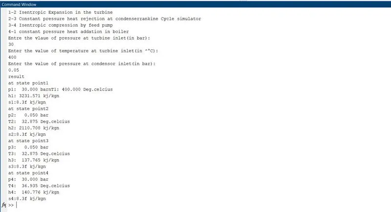
Error Faced :-
1) All the input are in stright line forget to add '\n'
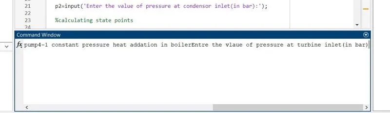
2) Typing mistake while function defination :-
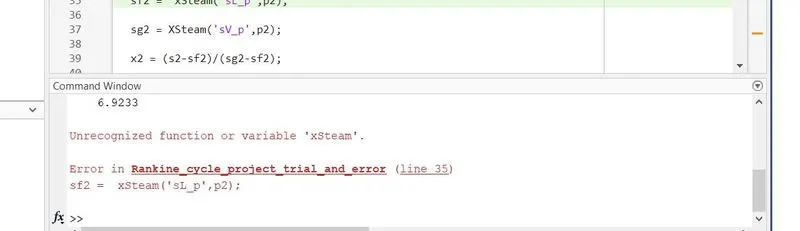
Getting Plot for T-S and H-S and Saturation curve :-
Plot for Temperature Vs Entropy:-
Plot for Enthalpy Vs Entropy :-
Conclusion :-
Getting sucessfully calculating state point values and getting plot for Temperature Vs Entropy and entropy Vs Entropy.