Challenge

Project 2 - Rankine cycle Simulator

SSunil K6 May 2022

Objective:

To Simulate a Rankine cycle using matlab.
Extracting Steam and water properties from XSteam data (IAPWS IF - 97 standard)
Calculating all the state points of the cycle based on User inputs.
Plotting the T vs s and H vs s plot for the given input.

Rankine Cycle:

Rankine cycle is an idealized thermodynamic cycle or heat engine in which a fuel is used to produce heat within a boiler , converting water into steam which then expands through a turbine producing useful wok . This process was developed in 1859 by scottish engineer william J.m Rankine . It is a cycle which converts heat into mechanical energy which usually is converted into electrical energy .
In this project an idealized cycle is simulated . Hence neglecting losses.
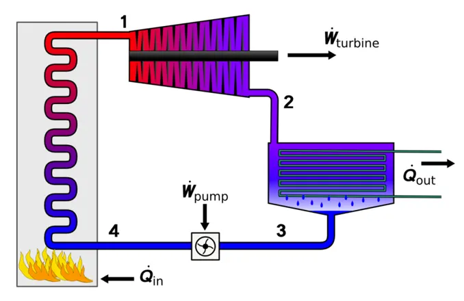
Rankine cycle is derived out of carnot cycle. its power depends on the temperature difference between the heat source and a cold source. The more the difference the more mechanical power can be efficiently extracted out of heat energy .
Since ideal cycles are only in theory , Efficiency of rankine cycle is limited by high heat of vaporization of the working fluid , friction losses etc.
Water is usually the fluid of choice due to its favorable properties, such as its non-toxic and unreactive chemistry, abundance, and low cost, as well as its thermodynamic properties. By condensing the working steam vapor to a liquid the pressure at the turbine outlet is lowered and the energy required by the feed pump consumes only 1% to 3% of the turbine output power and these factors contribute to a higher efficiency for the cycle. The benefit of this is offset by the low temperatures of steam admitted to the turbine

Processes and Working :

There are four processes in the rankine cycle (order maybe varied ) :

Process 1-2 : Isentropic Expansion in the turbine .
Process 2-3 : Constant pressure Heat rejection in condenser
Process 3-4 : Isentropic compression in the pump
Process 4-1 : Constant pressure heat addition in the boiler

Simulation code:

% rankine cycle simulator
% Objective of this program is to simulate the rankine cycle 
% Plotting t-s and h-s diagram using data from XSteam data
% Water and steam properties according to IAPWS IF-97  
clear all
close all
clc


disp(' RANKINE CYCLE ');                                    
disp('1-2 is Isentropic Expansion in the turbine');
disp('2-3 is constant pressure heat removal in the condenser');
disp('3-4 is Isentropic compression in the pump');
disp('4-1 is Constant pressure heat addition in the boiler');


%Obtaining the input data
p1 = input('nValue of pressure at turbine inlet, p1(in bar) = ');
T1 = input('nValue of temperature at turbine inlet, T1(in degree.C) = ');
p2 = input('nValue of temperature at condenser inlet, p2(in bar) = ');

% Extracting data _ defining variables
% State 1
h1 = XSteam('h_pT', p1, T1);        
s1 = XSteam('s_pT', p1, T1);        

% State 2-Isentropic expansion 
s2 = s1;                                           
sf2= XSteam('sL_p', p2);            
sg2 = XSteam('sV_p', p2);           
x2 = (s2-sf2)/(sg2-sf2);
hf2 = XSteam('hL_p', p2);           
hg2 = XSteam('hV_p', p2);
h2 = hf2 + (x2*(hg2-hf2));

% State 3-Constant pressure Heat rejection in condenser
p3 = p2;                            
s3= XSteam('sL_p', p3);
h3 = XSteam('hL_p', p3);

% State 4
s4 = s3;
p4 = p1;


% Work done by turbine
Wt = h1 - h2;

% Work done to run pump
v3 = XSteam('vL_p', p3);
Wp = v3*(p4 - p3)*100;
h4 = h3 + Wp;

%net work
Wnet = Wt - Wp;

%Heat into the system
Qin = h1 - h4;

%Heat out of the system
Qout = h2 - h3;

%Thermal efficiency
eff = (Wnet/Qin)*100;

%Specific Steam Consumption
%SSC = mass flow rate/power
SSC = (3600/Wnet);

%Calculating temperatures at the state points
T3 = XSteam('Tsat_p', p3);
T2 = T3;
Cp4 = XSteam('Cp_ps', p4, s4);
Cv4 = XSteam('Cv_ps', p4, s4);
k = Cp4/Cv4;
T4 = T3/((p3/p4)^((k-1)/k));

%Calculating temperature, entropy and enthalpy at the vapour and liquid
%line for plotting
T6 = XSteam('Tsat_p', p1);
s5 = XSteam('sL_p', p1);
s6 = XSteam('sV_p', p1);
h5 = XSteam('hL_p', p1);
h6 = XSteam('hV_p', p1);
T5 = T6;

%Plotting the saturation curve
T = linspace(1,375,1000);
for i = 1:length(T)

sf(i) = XSteam('sL_T', T(i));
sg(i) = XSteam('sV_T', T(i));
hf(i) = XSteam('hL_T', T(i));
hg(i) = XSteam('hV_T', T(i));
end

%Plotting T-s diagram
figure(1)
hold on
plot(sf, T, 'r','linewidth',1)
plot(sg, T, 'r','linewidth',1)
plot([s1 s2], [T1 T2], 'k', 'linewidth', 2)
plot([s2 s3], [T2 T3] ,'k', 'linewidth', 2)
plot([s3 s4], [T3 T4], 'k', 'linewidth', 2)
plot([s4 s5], [T4 T5], 'k', 'linewidth', 2)
plot([s5 s6], [T5 T6], 'k', 'linewidth', 2)
sc1 = linspace(s6, s1, 1000);
for l = 1:length(sc1)
 Tc1(l) = XSteam('T_ps', p1, sc1(l));
end
plot(sc1, Tc1, 'k', 'linewidth', 2)
text(s1+0.1, T1, '1')
text(s2+0.1, T2, '2')
text(s3, T3-20, '3')
text(s4, T4+20, '4')
title('Temp vs Entropy plot')
xlabel('Entropy ,S (Kj/kgk')
ylabel('Temperature (degree C) ')
legend('Saturation curve')


%Plotting h-s diagram
figure(2)
hold on
plot(sf, hf, 'r', 'linewidth', 1)
plot(sg, hg, 'r',  'linewidth', 1)
plot([s1 s2], [h1 h2], 'k', 'linewidth', 2)
plot([s2 s3], [h2 h3], 'k', 'linewidth', 2)
plot([s3 s4], [h3 h4], 'k', 'linewidth', 2)
hc = linspace(h4, h5, 100);
for k = 1:length(hc)
sch(k) = XSteam('s_ph', p1, hc(k));
end
plot(sch,hc, 'k', 'linewidth', 2)
plot([s5 s6], [h5 h6], 'k', 'linewidth', 2)
for m = 1:length(sc1)
hc1(m) = XSteam('h_ps', p1, sc1(m));
end
plot(sc1, hc1, 'k', 'linewidth', 2)
text(s1+0.1, h1, '1')
text(s2+0.1, h2, '2')
text(s3, h3-100, '3')
text(s4, h4 +200, '4')
title('Enthalpy vs Entropy plot')
xlabel('Entropy , S (KJ/kgk) ')
ylabel('Enthalpy , H (KJ/kg)')
legend('Saturation curve','location','northwest')

% Displaying Results
disp(' RESULTS');
fprintf('At State Point 1:n');
fprintf('p1: %8.3f barn', p1);
fprintf('T1: %8.3f Cn', T1);
fprintf('h1: %8.3f KJ/kgn', h1);
fprintf('s1: %8.3f KJ/kgKnn', s1);
fprintf('At State Point 2:n');
fprintf('p2: %8.3f barn', p2);
fprintf('T2: %8.3f Cn', T2);
fprintf('h2: %8.3f kJ/kgn', h2);
fprintf('s2: %8.3f kJ/kgKn', s2);
fprintf('x2: %8.3fnn', x2);
fprintf('At State Point 3:n');
fprintf('p3: %8.3f barn', p3);
fprintf('T3: %8.3f Kn', T3);
fprintf('h3: %8.3f kJ/kgn', h3);
fprintf('s3: %8.3f kJ/kgKnn', s3);
fprintf('At State Point 4:n');
fprintf('p4: %8.3f barn', p4);
fprintf('T4: %8.3f Kn', T4);
fprintf('h4: %8.3f KJ/kgn', h4);
fprintf('s4: %8.3f kJ/kgKnn', s4);
fprintf('Turbine Work: %8.3f kJ/kgn', Wt);
fprintf('Pump Work: %8.3f kJ/kgn', Wp);
fprintf('Wnet: %8.3f kJ/kgn', Wnet);
fprintf('Efficiency: %8.3f Percent n ', eff);
fprintf('S.S.C: %8.3f kJ/kWh', SSC);

Errors faced:

file directory error and file path.
spelling errors
printf errors and assigning units

Error rectification:

placed in a seperate file and path
checked the spelling and mathematical errors
written by hand then written on the code

References:

Project 2 - Rankine cycle Simulator

Ship work like this
in your own course.

Talk to a career counsellor

Ship work like thisin your own course.

Talk to a career counsellor

Ship work like this
in your own course.