Project 2 - Rankine cycle Simulator
OBJECTIVE: To code a MATAB program to create a rankinr cycle simulator and to calculate all the state points in it and als along with it plot th T-S and H-S diagram for the inputs given in th question.
THEORY
RANKINE CYCLE:
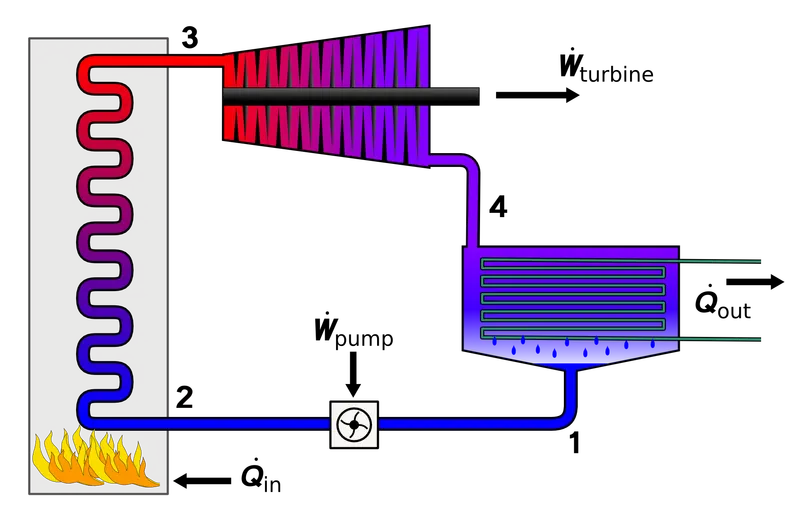
The Rankine cycle is an ideal thermodynamic cycle describing the process by which certain heat engines , such as steam turbines or reciprocating steam engines, allow mechanical work to be extracted from a fluid as it moves between a heat source and heat sink.
The Rankine Cycle’s major components include a rotating steam turbine, a boiler pump, a stationary condenser, and a boiler.A boiler is used to heat the water for steam at the required pressure and temperature as per the turbine’s requirement for power generation.The turbine exhaust is directed to the radial or axial flow condensor for condensing the steam to condensate and recycled back to the boiler through boiler pumps for heating again.
The 4 processes in rankine cycle are:
Process 1-2:
- Process 1-2: The working fluid is pumped from low to high pressure. As the fluid is a liquid at this stage, the pump requires little input energy. Process 1-2 is isentropic compression.
- Process 2-3: The high-pressure liquid enters a boiler, where it is heated at constant pressure by an external heat source to become a dry saturated vapour.Process 2-3 is constant pressure heat addition in boiler.
- Process 3–4: The dry saturated vapour expands through a turbine, generating power. This decreases the temperature and pressure of the vapour, and some condensation may occur.
- Process 4–1: The wet vapour then enters a condenser, where it is condensed at a constant pressure to become a saturated liquid. Process 4-1 is constant pressure heat rejection in condenser.
MAIN code
clear all
close all
clc
%displaying rankine cycle simulator and its processes
disp(" Rankine Cycle Simulator")
fprintf('1-2 is the isentropic expansion process')
fprintf('\n2-3 is the constant pressure heat rejection process')
fprintf('\n3-4 is the isentropic compression process')
fprintf('\n4-1 is the constant pressure heat addition process')
% State variables At state point 1
p1=30;
t1=400;
h1=Xsteam('h_pT',30,400);
s1=Xsteam('s_ph',30,h1);
fprintf('\n\n Results')
fprintf('\n\n At state point 1')
fprintf('\n P1 is:%f bar',p1)
fprintf('\n T1 is:%f deg celcius',t1)
fprintf('\n H1 is:%f KJ/Kg',h1)
fprintf('\n S1 is:%f KJ/KgK',s1)
% State variables At state point 2
p2=0.05;
s2=s1;
t2=Xsteam('T_ps',0.05,6.1858);
sf2=Xsteam('sL_p',p2);
sg2=Xsteam('sV_p',p2);
hf2=Xsteam('hL_p',p2);
hg2=Xsteam('hV_p',p2);
x=((s2-sf2)/(sg2-sf2));
h2=hf2+(x*(hg2-hf2));
v2=Xsteam('v_ph',p2,h2);
fprintf('\n\n At state point 2')
fprintf('\n P2 is:%f bar',p2)
fprintf('\n T2 is:%f deg celcius',t2)
fprintf('\n H2 is:%f KJ/Kg',h2)
fprintf('\n S2 is:%f KJ/KgK',s2)
% State variables At state point 3
p3=p2;
t3=t2;
h3=Xsteam('hL_T',32.875);
s3=Xsteam('sL_p',p3);
v3=Xsteam('v_ph',p3,h3);
fprintf('\n\n At state point 3')
fprintf('\n P3 is:%f bar',p3)
fprintf('\n T3 is:%f deg celcius',t3)
fprintf('\n H3 is:%f KJ/Kg',h3)
fprintf('\n S3 is:%f KJ/KgK',s3)
% State variables At state point 4
p4=p1;
s4=s3;
v4=v3;
h4=Xsteam('h_ps',p4,s4);
t4=Xsteam('T_hs',h4,s4);
fprintf('\n\n At state point 4')
fprintf('\n P4 is:%f bar',p4)
fprintf('\n T4 is:%f deg celcius',t4)
fprintf('\n H4 is:%f KJ/Kg',h4)
fprintf('\n S4 is:%f KJ/KgK',s4)
% State variables At state point 5
p5=p4;
t5=Xsteam('Tsat_p',p5);
h5=Xsteam('hL_T',t5);
s5=Xsteam('sL_p',p5);
fprintf('\n\n At state point 5')
fprintf('\n p5 is:%f bar',p5)
fprintf('\n T5 is:%f deg celcius',t5)
fprintf('\n H5 is:%f KJ/Kg',h5)
fprintf('\n S5 is:%f KJ/KgK',s5)
% State variables At state point 6
t6=t5;
p6=Xsteam('psat_T',t5);
h6=Xsteam('hV_T',t6);
s6=Xsteam('sV_T',t6);
fprintf('\n\n At state point 6')
fprintf('\n P6 is:%f bar',p6)
fprintf('\n T6 is:%f deg celcius',t6)
fprintf('\n H6 is:%f KJ/Kg',h6)
fprintf('\n S6 is:%f KJ/KgK',s6)
%loop to find variables on saturation lines
t=linspace(0,400,1000);
for i=1:length(t)
s_line1(i)=Xsteam('sL_T',t(i));
end
for j=1:length(t)
s_line2(j)=Xsteam('sV_T',t(j));
end
for i=1:length(t)
h_line1(i)=Xsteam('hL_T',t(i));
end
for j=1:length(t)
h_line2(j)=Xsteam('hV_T',t(j));
end
%net work output calculation
w_turbine=h1-h2;
w_pump=h4-h3;
work=w_turbine-w_pump;
q_in=h1-h4;
q_out=h2-h3;
%thermal efficiency
n=work/q_in;
%back work ratio
BWR=w_pump/w_turbine;
%specific steam consumption
ssc=3600/work;
%plottin T-s graph
figure(1)
hold on
plot([s_line1 s_line2],[t t])
plot([s1 s2 s3 s4 s5 s6 s1],[t1 t2 t3 t4 t5 t6 t1])
text(s1,t1,'1')
text(s2,t2,'2')
text(s3,t3,'3')
text(s4,t4,'4')
text(s5,t5,'5')
text(s6,t6,'6')
title('Rankine Cycle T-S diagram')
xlabel('Entropy(KJ/KgK)')
ylabel('Temperature(K)')
axis([0,8,0,450])
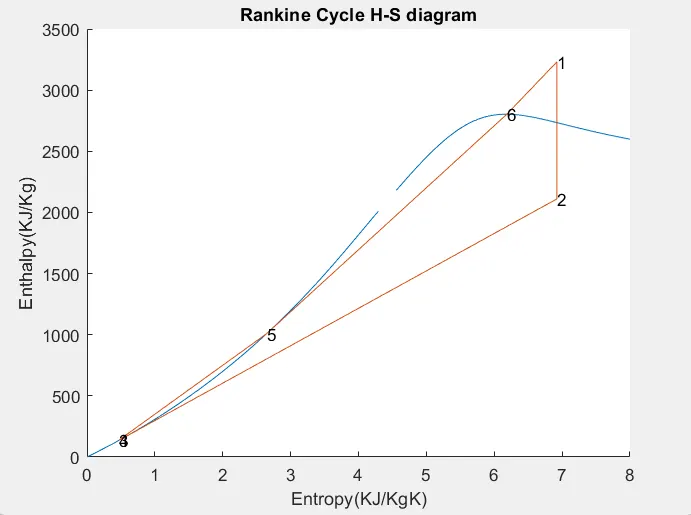
%plotting h-s graph
figure(2)
hold on
plot([s_line1 s_line2],[h_line1 h_line2])
plot([s1 s2 s3 s4 s5 s6 s1],[h1 h2 h3 h4 h5 h6 h1])
text(s1,h1,'1')
text(s2,h2,'2')
text(s3,h3,'3')
text(s4,h4,'4')
text(s5,h5,'5')
text(s6,h6,'6')
title('Rankine Cycle H-S diagram')
xlabel('Entropy(KJ/KgK)')
ylabel('Enthalpy(KJ/Kg)')
axis([0,8,0,3500])
Code explanation
Steps
- Firstly using the clear all, close all and clc to clear the command window data, workspace data and to close any opened plot windows.
- The dsp command is used to display the text 'Rankine cycle simulater and the processes associated with the rankine cycle is displayed using the fprintf command.
- The turbine inlet temperature is taken as 400K, the turbine inlet pressure is taken as 30 bar and the turbine outlet pressure is taken as 0.05 bar.
- The Xsteam.m file is put in the same path as the program and the xsteam function is called to find the state point values.
- The fprintf command is used to display the results in the command window.
- Using for loop to find the values for enthalpy and entropy at saturated temperature and stored them in variables.
- The net work done and the back work ratio are found using the respective formulas.
- From the values found the T-S and H-S diagrams are plotted.
- Lastly the saturation line also plotted.
RESULTS
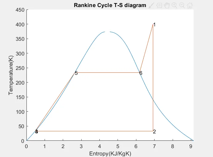
PLOT OF T-S
PLOT OF H-S
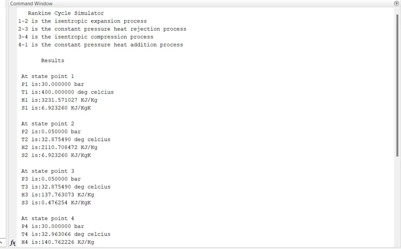
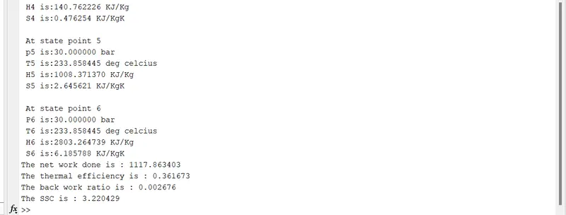
SCREENSHOT OF RESULTS DISPLAYED IN THE COMMAND WINDOW