Project 2 - Rankine cycle Simulator

PROJECT WORK 2

AIM-Rankine cycle simulator

% Rankine Cycle Simulator

clear all
close all
clc

% Display
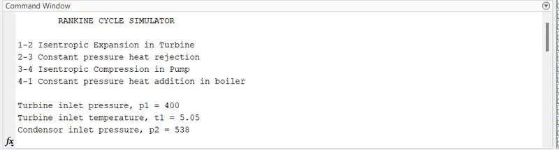
fprintf(' RANKINE CYCLE SIMULATOR\n\n')
fprintf('1-2 Isentropic Expansion in Turbine\n')
fprintf('2-3 Constant pressure heat rejection\n')
fprintf('3-4 Isentropic Compression in Pump\n')
fprintf('4-1 Constant pressure heat addition in boiler\n\n')

% User inputs
p1 = input('Turbine inlet pressure, p1 = ');
t1 = input('Turbine inlet temperature, t1 = ');
p2 = input('Condensor inlet pressure, p2 = ');
fprintf('\n')

% Calculations

% state 1
s1 = XSteam('s_pT',p1,t1);
h1 = XSteam('h_pT',p1,t1);

% state 2
t2 = XSteam('Tsat_p',p2);
s2 = s1;
sf2 = XSteam('sL_p',p2);
sg2 = XSteam('sV_p',p2);
hf2 = XSteam('hL_p',p2);
hg2 = XSteam('hV_p',p2);
x2 = ((s2-sf2)/(sg2-sf2));
h2 = hf2+(x2*(hg2-hf2));

% state 3
p3 = p2;
t3 = t2;
s3 = XSteam('sL_p',p3);
h3 = XSteam('hL_p',p3);
v3 = XSteam('vL_p',p3);

% state 4
p4 = p1;
s4 = s3;
cp4 = XSteam('Cp_ps',p4,s4);
cv4 = XSteam('Cv_ps',p4,s4);
g4 = cp4/cv4;
o = (g4-1)/g4;
t4 = t3*((p4/p3)^o);

% work done by pump
Wp = v3*(p4-p3)*100;

h4 = h3+Wp;

% state 5
s5 = XSteam('sL_p',p1);
h5 = XSteam('hL_p',p1);
t5 = XSteam('Tsat_p',p1);

% state 6
s6 = XSteam('sV_p',p1);
h6 = XSteam('hV_p',p1);
t6 = t5;

% work done by turbine
Wt = h1-h2;

% net work done
Wnet = Wt-Wp;

% Heat in
Qin = h1-h4;

% Heat out
Qout = h2-h3;

% Thermal efficiency
eff = Wnet/Qin;

% creating array for temperature
T = linspace(0,400,1000);

% entropy and enthalpy values for creating saturation curve
for i=1:length(T)
sf(i)=XSteam('sL_T',T(i));
sg(i)=XSteam('sV_T',T(i));
hf(i)=XSteam('hL_T',T(i));
hg(i)=XSteam('hV_T',T(i));
end

% T-S diagram
figure(1)
plot(sf,T)
hold on
plot(sg,T)
plot([s1,s2],[t1,t2],'Color','k')
plot([s2,s3],[t2,t3],'Color','k')
plot([s3,s4],[t3,t4],'Color','k')
plot([s4,s5],[t4,t5],'Color','k')
plot([s5,s6],[t5,t6],'Color','k')
plot([s6,s1],[t6,t1],'Color','k')
legend('Saturated Liquid','Saturated Vapour')
axis([0 8 0 450])
xlabel('Entropy(S)')
ylabel('Temperature(T)')
title('T-S diagram')

% H-S diagram
figure(2)
plot(sf,hf,'Color','r')
hold on
plot(sg,hg,'Color','r')
plot([s1,s2],[h1,h2],'Color','k')
plot([s2,s3],[h2,h3],'Color','k')
plot([s3,s4],[h3,h4],'Color','k')
plot([s4,s5],[h4,h5],'Color','k')
plot([s5,s6],[h5,h6],'Color','k')
plot([s6,s1],[h6,h1],'Color','k')
legend('Saturation curve')
axis([0 8 0 450])
xlabel('Entropy(S)')
ylabel('Entahlpy(H)')
title('H-S diagram')

% Back work ratio
Back_work_ratio = (h4-h3)/(h1-h2);

% SSC
SSC = 3600/(h1-h2);

% Displaying Results
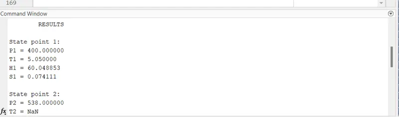
fprintf(' RESULTS\n\n')
fprintf('State point 1:\n')
fprintf('P1 = %f\n',p1)
fprintf('T1 = %f\n',t1)
fprintf('H1 = %f\n',h1)
fprintf('S1 = %f\n\n',s1)

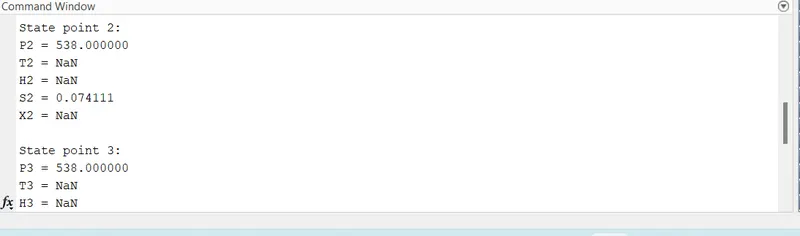
fprintf('State point 2:\n')
fprintf('P2 = %f\n',p2)
fprintf('T2 = %f\n',t2)
fprintf('H2 = %f\n',h2)
fprintf('S2 = %f\n',s2)
fprintf('X2 = %f\n\n',x2)

fprintf('State point 3:\n')
fprintf('P3 = %f\n',p3)
fprintf('T3 = %f\n',t3)
fprintf('H3 = %f\n',h3)
fprintf('S3 = %f\n\n',s3)

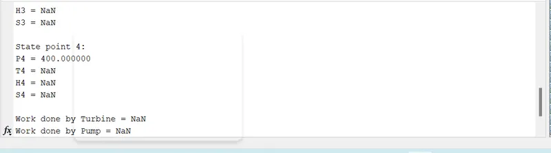
fprintf('State point 4:\n')

fprintf('P4 = %f\n',p4)
fprintf('T4 = %f\n',t4)
fprintf('H4 = %f\n',h4)
fprintf('S4 = %f\n\n',s4)

fprintf('Work done by Turbine = %f\n',Wt)
fprintf('Work done by Pump = %f\n',Wp)
fprintf('Net Work done = %f\n',Wnet)
fprintf('Thermal Efficiency = %f\n',eff)
fprintf('S.S.C = %f\n',SSC)

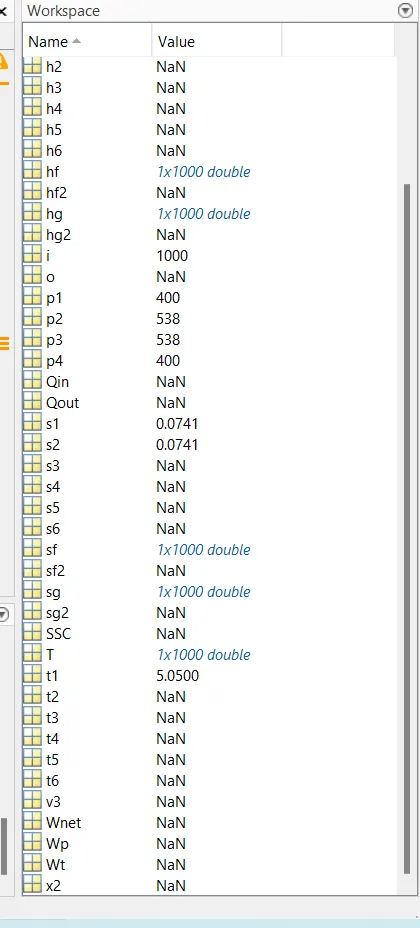
WORK SPACE SCREEN SHOTS