Project 2 - Rankine cycle Simulator
AIM:
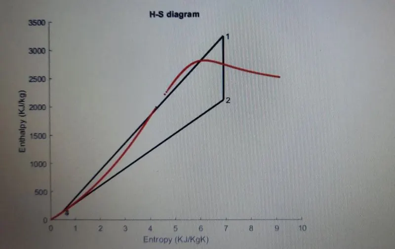
To create rankine cycle simulator using MATLAB. TO demonstrate the T-s and h-s plots for the given set of inputs.
OBJECTIVES:
. To create rankine cycle simulator using MATLAB.
. The code should calculate the state points of the Rankine cycle (any type of your choice) based on user inputs.
. The h-s plot and the T-s plot should be demonstrated based on the given input.
RANKINE CYCLE:
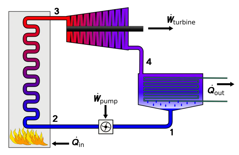
The Rankine cycle is an idealized thermodynamic cycle describing the process by which certain heat engines, such as steam turbines or reciprocating steam engines, allow mechanical work to be extracted from a fluid as it moves between a heat source and heat sink.
The Rankine cycle operates in the following steps:
1-2-3 Isobaric Heat Transfer.
- High pressure liquid enters the boiler from the feed pump.
- It is heated to the saturation temperature.
- Also addition of energy causes evaporation of the liquid until it is fully converted to saturated steam.
VARIOUS PROCESS OF RANKINE CYCLE:
The ideal Rankine cycle consists of the following four process:
1-2: Isentropic compression in a pump.
2-3: Constant pressure heat rejection in a boiler.
3-4: Isentropic expansion in a turbine.
4-1: Constant pressure heat rejection in a condenser.
TECHNICAL TERMS:
a) Enthalpy:
The enthalpy is the amount of heat content present in a system. It was denoted by 'h'.
b) Entropy:
Entropy is defined as a measure of randomness or disorder of a system. it was denoted by 's'.
FORMULA:
1. For Boiler:
Q1 = h1-hf4
2. For Turbine:
WT = h1-h2
3. For condenser:
Q2 = h2-hf3
4. For the feed pump:
Wp = hf4-hf3
5. Efficiency of the rankine cycle:
n = (h1-h2) - (hf4-hf3) / (h1-hf4)
When hf4 - hf3 value is very small then,
n = (h1 - h2) / (h1-hf4)
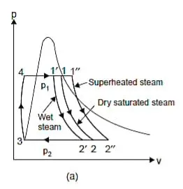
STEAM CONDITION:
It is consists of the following three process:
1) Wet steam (x<1)
2) Saturated steam (x=1)
3) Super saturated steam (x>1)
RANKINE CYCLE SIMULATOR CODE:
clear all
close all
clc
fprintf( 'RANKINE CYCLE SIMULATORn' )
fprintf(' 1-2 is Isentropic Expansion in turbinen' )
fprintf('2-3 is constent pressure heat rejection in condensorn')
fprintf('3-4 is Inentropic compression in pumpn')
fprintf('4-5 is constant pressure heat addition in boilern')
% Inputs
P1= input('turbine inlet pressure (bar)');
T1= input ('turbine inlet temperature (degree c)');
P2= input('turbine outlet pressure (bar)');
%Turbine inlet condition
T1- sat= Xsteam ('Tsat-p',P1);
if T1>T1-sat
h1= Xsteam (h'-pt',p1,T1);
s1= Xsteam('s-pt',p1,T1);
elseif T1==T1-sat
h1= Xsteam ('hv-p',p1);
s1= Xsteam ('sv-p',p1);
else
fprintf('enter higher temperature value')
end
%Turbine outlet condition
s2=s1;
s2-sat=Xsteam('sv-p',p2);
ifs2<s2-sat
s2-f =Xsteam('sl-p'.p2);
s2-g=Xsteam9'sv-p',p2);
x2=(s2 - s2-f)/(s2-g -s2-f);
h2-f=Xsteam('hL-p',p2);
h2-g=Xsteam('hv-p',p2);
h2=h2-f+x2*(h2-g -h2-f);
T2= Xsteam('Tsat-p',p2);
else
x2=1;
h2=Xsteam('hv-p',p2);
t2=Xsteam('Tsat-p',p2);
end
%condensor outlet condition
p3=p2;
T3=Xsteam('Tsat-p',p3);
h3=Xsteam('hL-p',p3);
s3=Xsteam('sL-p',p3);
v3=Xsteam('vL-p',p3);
%pump outlet condition
s4=s3;
p4=p1;
v4=Xsteam('v-ps',p4,s4);
cp=Xsteam('cp-ps',p4,s4);
cv=Xsteam('cv-ps',p4,s4);
g=cp/cv;
T4=T3*(p3/p4)^(1-g)/g));
w-p=v3*(p4-p3)*100;
h4=h3+w-p;
T5=Xsteam('Tsat-p',p4);
s5=Xsteam('sL-p',p4);
T6=T5;
s6=Xsteam('sv-T',T6);
%calculation of work done,heat and efficiency
w-t=h1-h2;
w-net=w_t -w_p;
Q_in=h1-h4;
Q_out=h2-h3;
efficiency=w_net/Q_in;
%Back work ratio calculation
ssc=3600/w_net;
%plotting
%T-s diagram
a=1 inspace(0,374,5000;
figure(1)
hold on
for i=1:length (a)
plot(Xsteam('SL_T',a(i))<a(i),'.',colour','r')
plot(Xsteam('sV_T",a(i)),a(i),'.','color','r')
plot([s1 s2],[T1 T2],'color','K','linewidth',2)
text(s1,T1,' 1')
text(s2,T2,' 2')
plot([s2 s6],[T1 T6],'color','K','linewidth' ,2)
plot([s6 s5],[T6 T6],'color', 'K', 'linewidth',2)
plot([s5 s4],[T6 T4],'color', 'K','linewidth' ,2)
text(s4, T4, '4' )
plot ([s4 s3],[T4 t3], 'color' , 'K', 'linewidth',2)
text(s3,T3, '3')
plot([s3 s1], [T3 T3], 'color', 'K', 'linewidth' ,2)
title(' T-S diagram')
xlable ('Entropy (KJ/Kgk)' )
ylable ('Temperature (Deg celcius)' )
%H-S diagram
figure (2)
hold on
plot([s1 s2], [h1 h2], ' color' , 'K', 'linewidth' ,2 )
text(s1,h1, ' 1')
text(s2,h2, ' 2')
plot([s2 s3], [h2 h3], 'color' , 'K' , 'linewidth' ,2)
plot([s3 s4],[h3 h4], 'color' , 'K' , 'linewidth' ,2)
text (s3,h3, ' 3')
text (s4,h4, ' 4')
text(s4,h4, ' 4')
plot([s4 s1],[h4 h1], 'color', 'K', 'linewidth' ,2)
for i=1:length (a)
plot (xsteam('sL_T' ,a(i)),xsteam('hL_T', a(i)), '.',' color' ,'r')
plot (xsteam('sv_T' ,a(i)),xsteam('hv_T' ,a(i)),'.','color' , 'r')
end
title('H-S diagram')
xlable('Entropy (KJ/Kgk) ')
ylable('Enthalpy(KJ/Kg) ')
%output
fprintf(' RESULTSn')
fprintf(' At state point 1: At state point 3:n')
fprintf(' %s %.2f', 'p1 is: ',p1, ' Bar ')
fprintf('%s %.2f' ,' P3 is : ',P3, ' Bar ')
fprintf( 'n' )
fprintf( '%s %2f' , 'T1 is : ',T1,' Deg celcius ')
fprintf('%s %.2f' ,' T3 is : ', T3 , ' Deg celcius ')
fprintf(' n' )
fprintf('%s %.2f ', 'H1 is : ',h1,' KJ/Kg')
fprintf('%s %2.f' ,' H3 is : ',h3, ' KJ/kg ')
fprintf('n ')
fprintf('%s %.2f' , 's1 is : ',s1,' KJ/Kgk' )
fprintf(' %s %.2f' ,' S3 is : ' , s3, ' KJ/ KgK ')
fprintf('nn')
fprintf('At state point 2: At state point 4:n')
fprintf('%s %.2f' , 'p2 is : ',p2, 'Bar')
fprintf('%s %.2f' ,' P4 is : ',P4, ' Bar ')
fprintf('n')
fprintf('%s %.2f' ,' T2 is: ' , T2, ' Deg celcius)
fprintf('%s %.2f' ,' T4 is : ', T4 , ' Deg celcius ')
fprintf('n')
fprintf('%s %.2f' ,' H2 is : ", h2,' KJ/Kg')
fprintf('%s %.2f' ,' H4 is : ',h4, ' KJ/kg ')
fprintf('n')
fprintf('%s %.2f ','s2 is : ', s2,' KJ/KgK')
fprintf('%S %.2f' ,' S4 is : ' , s4, ' KJ/ KgK ')
fprintf('nn')
fprint('%s %.2f' ,'wt is : ',W_t, ' KJ/kg')
fprintf('n')
fprintf('%s %.2f' ,'wp is :',W_P,' KJ/Kg')
fprintf('n')
fprintf('%s %.2f' ,'wnet is : ',W_net, ' KJ/Kg')
fprintf('n')
fprintf('%s %.2f' ,' Ntherm is : ',efficiency,' percent')
fprintf('n')
fprintf('%s %.2f' ,' S.S.C is : ', SSC,' KJ/ KWh')
fprintf('n')
fprintf('%s %.2f' ,'H2 is : ',h2,' KJ/Kg')
fprintf('%s %.2f' ,'
fprintf('n')
fprintf('%s %.2f' ,'s2 is : ', s2,' KJ/KgK')
fprintf('%s %.2f' ,'
fprintf('nn')
fprintf('%s %.2f' ,'Wt is : ',W_t,' KJ/Kg')
fprintf('n')
fprintf('%s %.2f' ,'Wp is :', W_p,' KJ/Kg')
fprintf('n')
fprintf('%s %.2f' ,'Wnet is :', W_net,' KJ/Kg')
fprintf('n')
fprintf('%s %.2f' ,'Ntherm is : ',efficiency, 'percent')
fprintf('n')
fprintf('%s %.2f' ,'S.S.C is :',SSC,' KJ/KWh')
fprintf('n')
Code explanation:
. Initially, the different process in a rankine cycle is displayed.
. The input parameters are obtained from the user.
. The different parameters at the turbine inlet condition is derived, The various constant values are obtained
. Here Xstream library is used for obtaining the steam table values.
. Then, the different parameters at turbine outlet condition is derived.
. In condenser outlet condition, different parameters are derived with the help of Xsteam library.
. The various values at the pump outlet condition are also calculated.
. Once the different values at different conditions are obtained, we can proceed further for calculating the main resultant values
. The work done, input and output heat and the efficiency of the rankine cycle is calculated.
. The back work ratio is also calculated.
. From all the values obtained the h-splot and the t-s plot were drawn
. All the values calculated are shown under result.
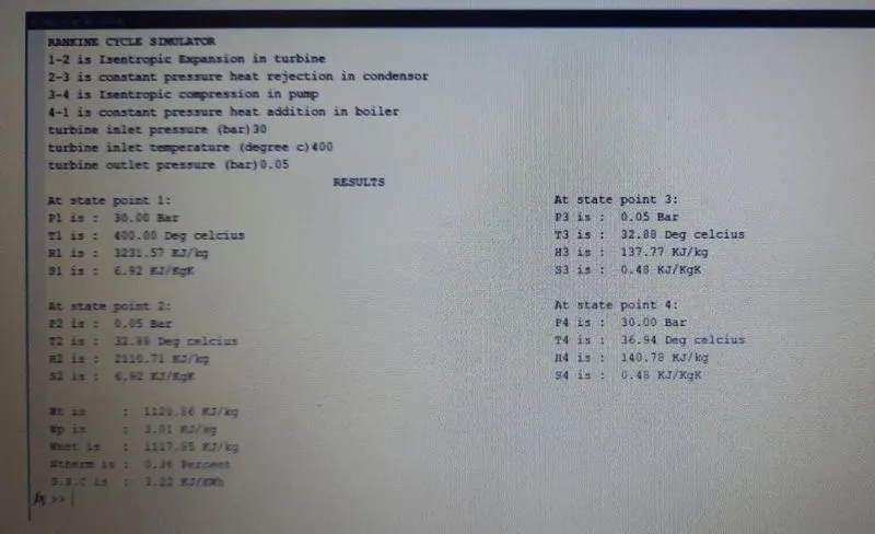
Input values:
. Turbine inlet temperature=400'C
. Turbine inlet pressure=30bars
. Turbine outlet pressure=0.005bars= Condenser inlet pressure.
OUTPUT VALUES:
Result values:
The various result values calculated for the given input is shown below,
Results plots:
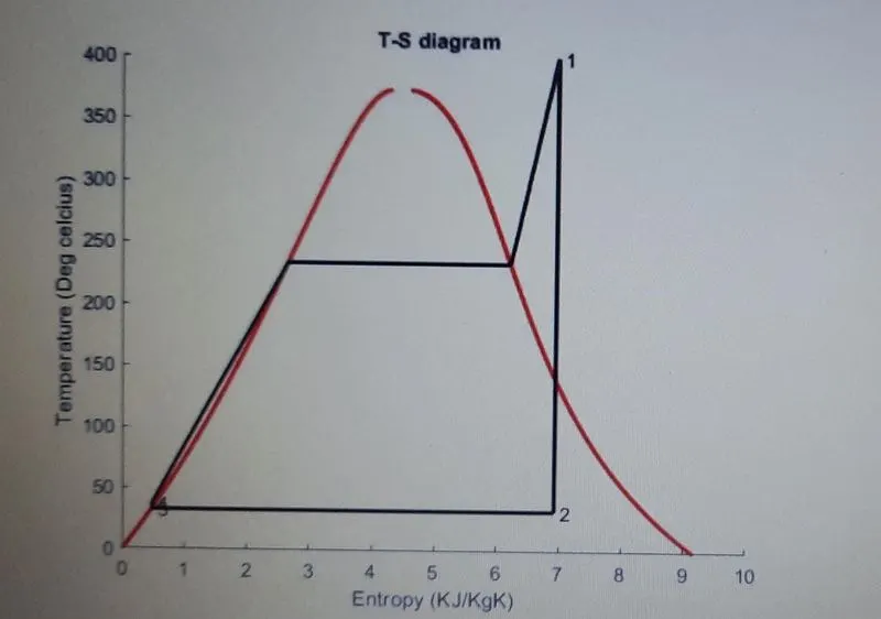
Conclusion:
Thus the result of rankine cycle simulator was made using MATLAB. Thus the result of the input parameters and plots are shown.