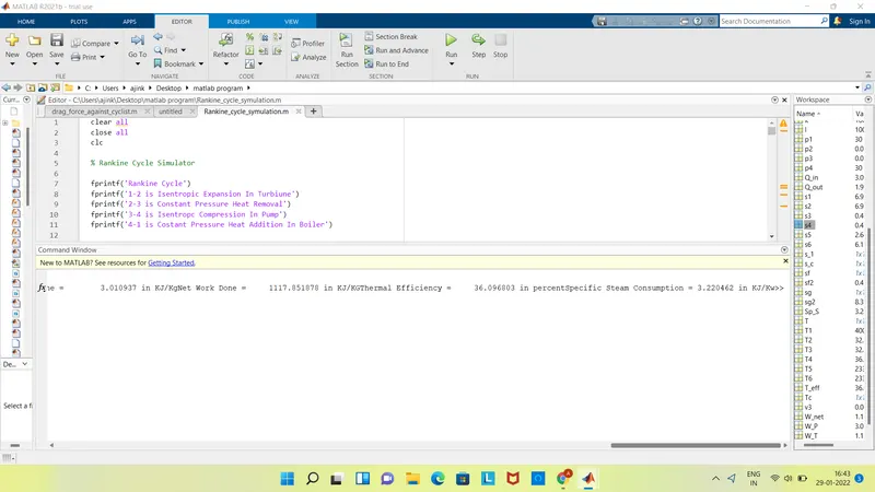
Project 2 - Rankine cycle Simulator

clear all
close all
clc

% Rankine Cycle Simulator

fprintf('Rankine Cycle')
fprintf('1-2 is Isentropic Expansion In Turbiune')
fprintf('2-3 is Constant Pressure Heat Removal')
fprintf('3-4 is Isentropc Compression In Pump')
fprintf('4-1 is Costant Pressure Heat Addition In Boiler')

% Input Data
% Temprature at Turbine Inlet
T1 = 400;
% Pressure at Turbine Inlet 
p1 = 30;
% Pressure at Condenser
p2 = 0.05;

% Taking data from Xsteam file for state point 1
% Enthalpy at pressure and Temp 1
h1 = XSteam('h_pT', p1, T1);
% Entropy at pressure and Temp 1
s1 = XSteam('s_pT', p1, T1);

% Taking data from Xsteam file for state point 2
% Because of Isentropic Expansion
s2 = s1;
% Saturated liquid entropy at pressure 2
sf2 = XSteam('sL_p', p2);
% Saturated vapour entropy at pressure 2
sg2 = XSteam('sV_p', p2);
% Vapour fraction
x2 = (s2-sf2)/(sg2-sf2);
% Saturated liquid enthaply at pressure 2
hf2 = XSteam('hL_p', p2);
% Saturated vapour enthalpy at pressure 2
hg2 = XSteam('hV_p', p2);
% Enthaply at state point 2
h2 = hf2 + (x2*(hg2-hf2));


% Taking data from Xsteam file for state point 3
% Because of canstant pressure heat removal process
p3 = p2;
% Saturated liquid entropy at pressure 3
s3 = XSteam('sL_p', p3);
% Saturated liquid enthaply at pressure 3
h3 = XSteam('hL_p', p3);



% Taking data from Xsteam file for state point 4
% Because of isentropic compression process
s4 = s3;
% Because of constant pressure heat rejection
p4 = p1;

% Work done in Turbine for Rankine Cycle
W_T = h1-h2;

% Work done required for pump
% Saturated liduid vapour at pressure 3
v3 = XSteam('vL_p', p3);
% Work done for pump
W_P = v3*(p4-p3)*100;
% Enthaply at state point 4
h4 = h3 - W_P;

% Net work done for Rankine Cycle
W_net = W_T -W_P;

% Heat Addition to System
Q_in = h1-h4;

% Heat Rejection from system
Q_out = h2-h3;

% Thermal Efficincy of Rankine Cycle
T_eff = (W_net/Q_in)*100;

% Specific Steam consumption
Sp_S = (3600/W_net);

% Calculation of Temp at All state point 2, 3 and 4
% Saturation Temp at pressure 3
T3 = XSteam('Tsat_p',p3);
% Constant Pressure heat addition
T2 = T3;
% Specific Isobaric heat capacity
Cp4 = XSteam('Cp_ps',p4,s4);
% Specific Isochoric heat capacity
Cv4 = XSteam('Cv_ps',p4,s4);
k = Cp4/Cv4;
% Temperature at state point 4
T4 = T3/((p3/p4)^((k-1)/k));


% Calculation of other constant for saturated liquid and vapour
% Saturated Temperature at pressure 1
T6 = XSteam('Tsat_p', p1);
% Saturated Liquid entropy at pressure 1
s5 = XSteam('sL_p', p1);
% Saturated Vapour entropy at pressure 1
s6 = XSteam('sV_p', p1);
% Saturated liquid enthalpy at pressure 1
h5 = XSteam('hL_p', p1);
% Saturated Vapour enthalpy at pressure 1
h6 = XSteam('hV_p', p1);
T5 = T6;

% Plotting for Saturation Line
T = linspace(1,560,1000);
for i = 1:length(T)
    sf(i) = XSteam('sL_T', T(i));
    sg(i) = XSteam('sV_T', T(i));
    hf(i) = XSteam('hL_T', T(i));
    hg(i) = XSteam('hV_T', T(i));
end


% Plotting T-S Diagram or Rankine Cycle
figure(1)
hold on
plot(sf,T,'Color','b','LineWidth',3)
plot(sg,T,'Color','b','LineWidth',3)
plot([s1 s2],[T1 T2], 'Color','r','LineWidth',4)
plot([s2 s3],[T2 T3], 'Color','r','LineWidth',4)
plot([s3 s4],[T3 T4], 'Color','r','LineWidth',4)
plot([s4 s5],[T4 T5], 'Color','r','LineWidth',4)
plot([s5 s6],[T5 T6], 'Color','r','LineWidth',4)
s_1 = linspace(s6,s1,1000);
for j = 1:length(s_1)
    Tc(j) = XSteam('T_ps',p1,s_1(j));
end

plot(s_1,Tc,'Color','r','LineWidth',4)
text(s1+0.1, T1, '1')
text(s2+0.1, T2, '2')
text(s3, T3-20, '3')
text(s4, T4+20, '4')
title('Temperature Vs Entropy')
xlabel('Entropy (Kj/kg-k)')
ylabel('temperature(Deg. Celcius)')
legend('Satuyration Curve')

% Plotting H-S Diagram for Rankine Cycle
figure(2)
hold on
plot(sf,hf,'Color','b','LineWidth',3)
plot(sg,hg,'Color','b','LineWidth',3)
plot([s1 s2],[h1 h2],'Color','r','LineWidth',4)
plot([s2 s3],[h2 h3],'Color','r','LineWidth',4)
plot([s3 s4],[h3 h4],'Color','r','LineWidth',4)
hc = linspace(h4,h5,100);
for k = 1:length(hc)
    s_c(k) = XSteam('s_ph',p1,hc(k));
end

plot(s_c,hc,'Color','r','LineWidth',4)
plot([s5 s6],[h5 h6],'Color','r','LineWidth',4)
for l = 1:length(s_1)
    h_c(1) = XSteam('h_ps',p1,s_1(1));
end

plot(s_1,h_c,'Color','r','LineWidth',4)
text(s1+0.1,h1,'1')
text(s2+0.1,h2,'2')
text(s3,h3-100,'3')
text(s4,h4+200,'4')
title('Enthalpy Vs Entropy')
xlabel('Entropy (Kj/kg-k)')
ylabel('Enthalpy (Kj/kg)')
legend('Saturation Curve')

% Displaying Results In Command Window
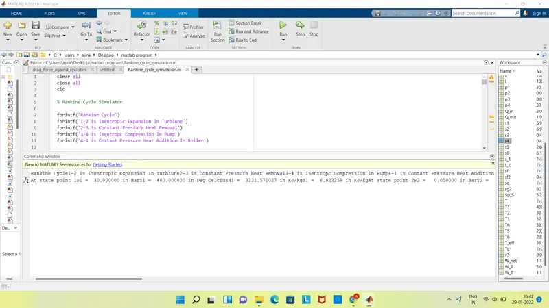
disp('Results of Rankine Cycle')
fprintf('At state point 1')
fprintf('P1 = %10f in Bar',p1);
fprintf('T1 = %11f in Deg.Celcius',T1);
fprintf('H1 = %12f in KJ/Kg',h1);
fprintf('S1 = %9f in KJ/Kg',s1);

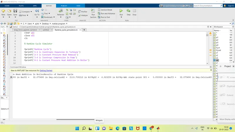
fprintf('At state point 2')
fprintf('P2 = %10f in Bar',p2);
fprintf('T2 = %11f in Deg.celcius',T2);
fprintf('H2 = %12f in KJ/Kg',h2);
fprintf('S2 = %9f in KJ/Kg-k',s2);

fprintf('At state point 3')
fprintf('P3 = %10f in Bar',p3);
fprintf('T3 = %11f in Deg.Celcius',T3);
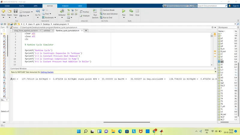
fprintf('H3 = %12f in KJ/Kg',h3);
fprintf('S3 = %9f in KJ/Kg',s3);

fprintf('At state point 4')
fprintf('P4 = %10f in Bar',p4);
fprintf('T4 = %11f in Deg.celcius',T4);
fprintf('H4 = %12f in KJ/Kg',h4);
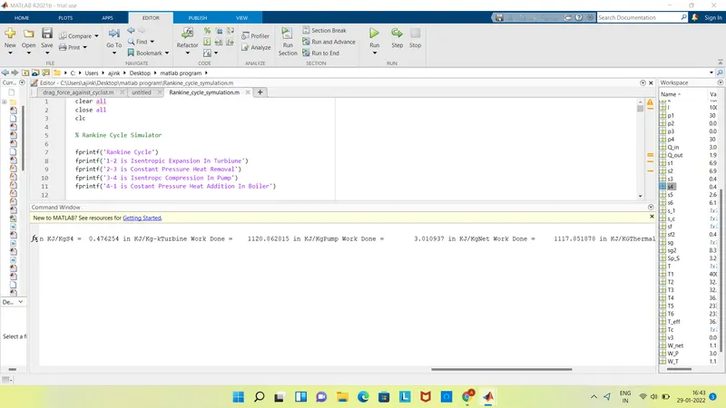
fprintf('S4 = %9f in KJ/Kg-k',s4);


fprintf('Turbine Work Done = %14f in KJ/Kg',W_T)
fprintf('Pump Work Done = %15f in KJ/Kg',W_P)
fprintf('Net Work Done = %15f in KJ/KG',W_net)
fprintf('Thermal Efficiency = %13f in percent',T_eff)
fprintf('Specific Steam Consumption = %f in KJ/Kw',Sp_S)

Report

The Rankine Cycle is thermodynamic cycle.It cinvert heat energy into mechanical workby undergoing phase change.Heat energy is supplied externally to the system.Rnakine cycle has four component like wise pump,boiler,turbine,condeser.Water is used as a working fliud.

Process involve in Rankine Cycle :

1. Isentropic Expansion in turbine

2. Constant pressure heat rejection

3. Isentropic compression in pump

4. Constant pressure heat addition

Code Explianation:

fprintf : To display result of cycle simulation in command window.

Input variables p1, T1, p2 are provieded by input command.Values of entropy and enthalpy is extracted from Xsteam file.

Work done , Thermal efficiency and specific steam consumption is calculated using basic formulas.

For saturation curve temprature range is defined using linspace command.

Potting of H-S and T-S digram is done by using plot command.

Results:

l