Project 2 - Rankine cycle Simulator
Aim : To develop a code to simulate basic Rankine Cycle.
Objective :
1.To develop a code to determine the state variables for various states of a basic Rankine Cycle with the given parameters i.e. pressure and temperature at turbine inlet and pressure at the condenser inlet.
2. Output of all the state variables and mechanical properties.
3. Plot the T-S and H-S diagram with the obtained results along with saturated pressure lines.
Theory :
A Rankine Cycle is an idealised cycle for a steam plant consisting of boiler, turbine , condenser and feed pump. The cycle has four fundamental ideal process which are:
1-2 : Isentropic Expansion (in turbine)- The vapor is expanded in the turbine, thus producing work which may be converted to electricity. Depending upon the turbine efficiency and number of stages the steam can leave in the form of vaopur or it can get condensed and a mixture of vapour and liquid can be given as output. To know the state of the steam the entropy is compared and the dryness fraction is calculated accordingly.
2-3 : Constant Pressure Heat Rejection (in condenser) - The vapour or vapor-liquid mixture leaving the turbine is condensed at by reducing its temperature at a low pressure and liquid water is given as outlet.
3-4 : Isentropic Compression (pump) - The pressure of the water is then raised in the feed pump.
4-1 : Constant Pressure Addition (in boiler)- The high pressure liquid from the pump enters the boiler, which is heated till its saturation temperature and converted into steam.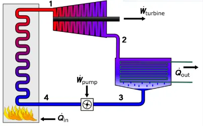
The working fluid for the rankine cycle in a steam power plant is water and steam. The steam can be classified as saturated and superheated steam on the basis of its temperature and pressure. According to the pressure the properties like specific volume, enthalpy, entropy can be determined with the help of steam tables.
Based on the nature of steam states for saturated and superheated steam intermidiate points can be determined. The basic terminology used for the calculation is :
a) Saturation Pressure - Pressure at which liquid and vapour co-exists in equllibrium at a given temperature. Ex- Saturation pressure for water at 100 deg celcius is 1 atm.
b)Saturation Temperature – Temperature at which the liquid liquid starts boiling at a given pressure. Ex- Saturation temperature for water at 1 atm pressure is 100 deg celcius.
c) Af - Property A at saturated liquid state. Ex- Sf, Hf, Vf.
d)Ag - Property A at saturated vapour state . Ex- Sg, Hg, Vg.
e)Afg – Change in property A while changing phase from liquuid to water.
f) Dryness fraction (x) – It is the ratio of the mass of vapour to the total mass of vapour and liquid mixture.
Code Syntax :
XSteam is a function which is used to determine the values for different variables. The syntax for the various function used in the code are-
Variable = XSteam(‘steam function handle’,Argument 1, Argument 2);
XSteam takes two or three arguments, the first argument is the steam function and the later two are the inputs to that particualr steam function, this will give desired value which will be stored in the assigned variable. Different steam function used in the code were:
• Tsat_p - Saturation temperature as a function of pressure.
• hV_p - Saturated vapour enthalpy as a function of pressure.
• hL_p - Saturated liquid enthalpy as a function of pressure.
• h_ps - Entalpy as a function of pressure and entropy as a function of pressure and entropy.
• h_pT - Entalpy as a function of pressure and temperature.
• h_ps - Entalpy as a function of pressure and entropy.
• hV_T - Saturated vapour enthalpy as a function of temperature.
• hL_T -Saturated liquid enthalpy as a function of temperature.
• sV_T - Saturated vapour entropy as a function of temperature.
• sL_T - Saturated liquid entropy as a function of temperature.
• sV_p - Saturated vapour entropy as a function of pressure.
• sL_p - Saturated liquid entropy as a function of pressure.
• s_pT - Specific entropy as a function of pressure and temperature (Returns saturated vapour entalpy if mixture.)
• CpV_p - Saturated vapour heat capacity as a function of pressure
• CpL_p - Saturated liquid heat capacity as a function of pressure.
• CvV_p - Saturated vapour isochoric heat capacity as a function of pressure.
• CvL_p - Saturated liquid isochoric heat capacity as a function of pressure.
Algorithm :
1. Taking the inputs for the pressure and temperature at turbine inlet, pressure at condenser inlet.
2. Getting specific heat capacity values for saturated liquid and vapour.
3. Getting specific entropy and specific enthalpy data from Xsteam for the variables at state 1 for saturated liquid and vapour states.
4. Getting specific entropy and specific enthalpy data from Xsteam for the variables at state 2 for saturated liquid and vapour states.
5. Calculating state 3 variables.
6. Calculating state 4 variables.
7. Calculation of work done by turbine, condenser , net work and back work ratio.
8.Calculation for the effficiency and ssc.
9. Getting values for satutrated lines as a function of temperature.
10. Printing the output for all state variables and mechanical properties.
11. Plotting the H-S and T-S diagram.
Main Code :
clear all
close all
clc

%INPUT FOR THE INITIAL STATE

%Turbine inlet pressure (Bar)
p1=input ('Enter the pressure at the Turbine Inlet(in bar): ');
%Turbine inlet temperature (Deg Celcius)
t1=input ('Enter the temperature at the Turbine Inlet( in kelvin): ');
%Turbine outlet pressure (Bar)
p2=input ('Enter the pressure at the condenser(in bar): ');

%GETTING DATA FROM XSTEAM
CPg2=XSteam('CpV_p', p2);  %specific heat vapour
CPf1=XSteam('CpL_p', p1);  %specific heat fluid

%GETTING DATA FOR STATE 1
t1s=XSteam('Tsat_p',p1); %saturation temperature for p1 at point 1s
s1g=XSteam('sV_p',p1);   %entropy at point 1s
s1f=XSteam('sL_p',p1);   %entropy at point 4s
h1g=XSteam('hV_p',p1);   %enthalpy at point 1s
h1f=XSteam('hL_p',p1);   %enthalpy at point 4s

%Parameters for the phase change
h1fg=h1g-h1f; %enthalpy change of phase change
s1fg=s1g-s1f; %entropy change of phase change

h1=XSteam('h_pT',p1,t1); %enthalpy at point 1
s1=XSteam('s_pT',p1,t1); %entropy at point 1

%GETTING DATA FOR STATE 2
t2s=XSteam('Tsat_p',p2); %temperature at point 2s
h2g=XSteam('hV_p',p2);   %enthalpy at point 2s
h2f=XSteam('hL_p',p2);   %enthalpy st point 3
s2g=XSteam('sV_p',p2);   %entropy at point 2s
s2f=XSteam('sL_p',p2);   %entropy at point 3

s2fg=s2g-s2f; %entropy change of phase change
h2fg=h2g-h2f; %enthalpy change of phase change

s2=s1;        %entropy for state 2

%Comparing the entropy and determinig dryness fraction
if(s2<=s2g)
   x=((s2-s2f)/(s2fg));
else
   x=1;
end

%Calculating temperature and enthalpy for state 2
if(x<1)
  t2=t2s;
  h2=h2f+x*h2fg;
 else
  t2=(t2s+273.15)*exp((s2-s2g)/CPg2);
  t2=t2-273.15;
  h2=h2g+CPg2*(t2-t2s);
end

%DATA FOR STATE 3
p3=p2;   %pressure at point 3
t3=t2s;  %temperature at point 3
h3=h2f;  %enthalpy at point 3
s3=s2f;  %entropy at point 3

%DATA FOR STATE 4
p4=p1;   %pressure at point 4
s4=s3;   %entropy at point 4
t4=t1s/(exp((s1f-s4)/CPf1));  %temperature at point 4
h4=XSteam('h_ps',p4,s4);      %enthaply at point 4


%CALCULATION OF WORK DONE
wt=h1-h2;    %work done by turbine
wp=h4-h3;    %work done by pump
bw=wp/wt;    %back work ratio
wnet=wt-wp;  %net work done

%CALCULATION OF EFFICIENCY AND SSC
q_in=h1-h4;           %heat addition
q_out=h2-h3;          %heat rejection
n=100*(wnet/q_in);    %efficiency
ssc=3600/wnet;        %specific steam consumption

%CALCULATION FOR SATURATED LINE
temp=linspace(0,400,400);
for i=1:length(temp)

  h_f(i)=XSteam('hL_T',temp(i)); %saturated liquid line for enthalpy
  h_g(i)=XSteam('hV_T',temp(i)); %saturated vapour line for enthalpy
  s_f(i)=XSteam('sL_T',temp(i)); %saturated liquid line for entropy
  s_g(i)=XSteam('sV_T',temp(i)); %saturated vapour line for entropy

end

%PRINTING STATEMENT FOR PATHS
printf('*****RANKINE CYLE SIMULATOR****\n\n')
printf(' 1-2 ISENTROPIC eXPANSION IN THE TURBINE\n' )
printf(' 2-3 CONSTANT PRESSURE HEAT REJECTION \n')
printf(' 3-4 ISENTROPIC COMPRESSION IN THE PUMP \n')
printf(' 4-1 CONSTANT PRESSURE HEAT ADDITION \n\n')

%PRINTING OUTPUT AT STATE 1
printf('*****RESULTS*****\n\n')
printf('At State point 1: \n')
printf('P1 is : %f Bar \n',p1)
printf('T1 is : %f Deg Celcius \n',t1)
printf('H1 is : %f kJ/kg \n',h1)
printf('S1 is : %f kJ/kgK \n\n',s1)

%PRINTING OUTPUT AT STATE 2
printf('At State point 2: \n')
printf('P2 is : %f Bar \n',p2)
printf('T2 is : %f Deg Celcius \n',t2)
printf('H2 is : %f kJ/kg \n',h2)
printf('S2 is : %f kJ/kgK \n',s2)
printf('X2 is : %f\n\n',x)

%PRINTING OUTPUT AT STATE 3
printf('At State point 3: \n')
printf('P3 is : %f Bar \n',p3)
printf('T3 is : %f Deg Celcius \n',t3)
printf('H3 is : %f kJ/kg \n',h3)
printf('S3 is : %f kJ/kgK \n\n',s3)

%PRINTING OUTPUT AT STATE 4
printf('At State point 4: \n')
printf('P4 is : %f Bar \n',p4)
printf('T4 is : %f Deg Celcius \n',t4)
printf('H4 is : %f kJ/kg \n',h4)
printf('S4 is : %f kJ/kgK \n\n',s4)

%PRINTING OUTPUT FOR WORK AND EFFICIENCY
printf('Wt is   : %f kJ/kg\n',wt)
printf('Wp is   : %f kJ/kg\n',wp)
printf('Back work ratio : %f\n',bw)
printf('Wnet is : %f kJ/kg\n',wnet)
printf('Ntherm is : %f Percent\n',n)
printf('Specific steam consumption is : %f kg/kWh\n',ssc)

%PLOTTING RANKINE CYCLE
%PLOTTING T-S DIAGRAM
figure(1)
hold on

plot([s1 s2],[t1 t2],'color','k')
plot([s2 s2g],[t2 t2s],'color','k')
plot([s2g s3],[t2s t3],'color','k')
plot([s3 s4],[t3 t4],'color','k')
plot([s4 s1f],[t4 t1s],'color','k')
plot([s1g s1],[t1s t1],'color','k')
plot([s1f s1g],[t1s t1s],'color','k')
%Plotting saturated line
plot(s_f,temp,'color','r')
plot(s_g,temp,'color','r')
%Marking points
text(s1,t1,'1')
text(s1g,t1s,'1s')
text(s2,t2,'2')
text(s2g,t2s,'2s')
text(s3,t3,'3')
text(s4,t4,'4')
text(s1f,t1s,'4s')
%Label and titles
xlabel('Entropy [kJ/kgK]')
ylabel('Temperature [Deg Celcius]')
title('T-S Diagram')

%PLOTTING H-S DIAGRAM
figure(2)
hold on

plot([s1 s2],[h1 h2],'color','k')
plot([s2 s3],[h2 h3],'color','k')
plot([s3 s4],[h3 h4],'color','k')
plot([s4 s1],[h4 h1],'color','k')
%Plotting saturated line
plot(s_f,h_f,'color','r')
plot(s_g,h_g,'color','r')
%Marking points
text(s1,h1,'1')
text(s2,h2,'2')
text(s3,h3,'3')
text(s4,h4,'4')
%label and titles
xlabel('Entropy [kJ/kgK]')
ylabel('Enthalpy [kJ/kg]')
title('H-S Diagram')
Error : There were several syntax errors that occured while writing the code which were resloved by refering to the XSteam file and matlab resources.
Conclusion :
The output of all state variables is displayed and the required plots for the TS and HS diagram are obtained. The transition between the states are represented by assuming the specific heat to be constant for whole process. For project work can be extened further by including the preheater, superheater, economiser and multiple turbine stages. A more accurate representation can be made by taking account of the change in specific heat capacity.
References :