Project 2 - Rankine cycle Simulator

AIM : Create Rankine cycle simulater using MATLAB and to calculate net work output , back work ratio.

THEORY :

The ideal Rankine cycle consists of the following four processes.

• 1-2 isentropic expansion in teh turbine.
• 2-3 constant pressure heat rejection in a condensor.
• 3-4 isentropic compression in a compressor.
• 4-1 constant pressure heat addition in a bolier.

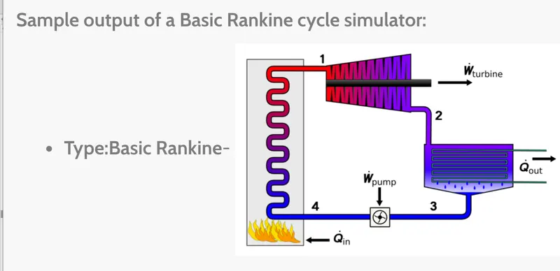
Turbine(process1-2) :

Steam from the boiler ,which has an elevated temperature and pressure ,expands through the turbine to produce work and then is discharged to the condensor with relatively low pressure.

W(turbine.out) = h2 - h1

Condensor(2-3) :

Steam from the turbine is condensed to liquid in the condenser. The energy balance in condensor is

Qout = h2 - h3

Pump(process 3-4) :

Pump pressurized the liquid water from the condenser prior to going back to the bolier .Assuming no heat transfer with the surroundings the energy balance in the pump is

Wpump in = h4 - h3

Boiler(process 2-3):

Liquid water enters the boiler and is heated to superheated state in the boiler.The energy balance in the boiler is

Qin =h1 - h4

MATLAB CODE:

clear all
close all
clc


disp('       RANKINE CYCLE SIMULATOR');
disp('1-2 is isentropic exoansion in the turbine');
disp('2-3 is isochoric heat removal in thr condenser');
disp('3-4 is isentropic compression in the pump');
disp('4-1 is isochoric heat addition in the boiler');

%obtaining the input data

% value of pressure at turbine inlet in bar

p1 = 30;

%value of temperature at turbine inlet in C
T1 = 400;

%value of pressure at condenser inlet in bar
p2 = 0.05;

% At stage 1
h1 = XSteam('h_pT', p1, T1);
s1 = XSteam('s_pT', p1,T1);

%stage 2 
%s2 = sf2-x(sfg2)

s2 =s1;

sf2 = XSteam('sL_p',p2);
sg2 = XSteam('sV_p',p2);
x2 = (s2-sf2)/(sg2-sf2);

hf2 = XSteam('hL_p',p2);
hg2 = XSteam('hV_p',p2);
h2 = hf2 + (x2*(hg2-hf2));


%At stage 3

p3 = p2;

s3 = XSteam('sL_p',p3);

h3 = XSteam('hL_p',p3);

%At stage 4

s4 = s3;
p4 = p1;

% work done at turbine
Wt = h1 -h2;

%work done to run pump 
v3 =XSteam('vL_p',p3);
Wp = v3*(p4-p3)*100;
h4 = h3 + Wp;

%net work

Wnet = Wt - Wp;

%heat into the system

Qin = h1 + h4;

%heat out of the system
Qout = h2 -h3;

%thermal efficiency 

eff = (Wnet/Qin)*100;

%specific steam consumption 
%ssc = mass flow rate/power

SSC = (3600/Wnet);


% calculating temperatures at the state points
T3 = XSteam('Tsat_p',p3);
T2 = T3;
Cp4 = XSteam('Cp_ps',p4,s4);
Cv4 = XSteam('Cv_ps',p4,s4);
k = Cp4/Cv4;
T4 = T3/((p3/p4)^((k-1)/k));

%calculating temperature ,entropy and enthalpy

T6 = XSteam('Tsat_p',p1);
s5 = XSteam('sL_P',p1);
s6 = XSteam('sV_p',p1);
h5 = XSteam('hL_p',p1);
h6 = XSteam('hV_p' ,p1);
T5 =T6;

%plotting 

T = linspace(1,375,1000);

for i = 1:length(T)
    sf(i) = XSteam('sL_T',T(i));
    sg(i) = XSteam('sV_T',T(i));
    hf(i) = XSteam('hL_T',T(i));
    hg(i) = XSteam('hV_T',T(i));
end

%plotting T-s diagram

figure(1)
hold on
plot(sf,T,'r');
plot(sg,T,'r');
plot([s1 s2],[T1 T2],'b','linewidth',3);
plot([s2 s3],[T2 T3],'b','linewidth',3);
plot([s3 s4],[T3 T4],'b','linewidth',3);
plot([s4 s5],[T4 T5],'b','linewidth',3);
plot([s5 s6],[T5 T6],'b','linewidth',3);

sc1 = linspace(s6,s1,1000);
for l = 1:length(sc1)

    Tc1(1) = XSteam('T_ps',p1,sc1(1));
end

plot(sc1,Tc1,'b','linewidth',3);
text(s1+0.1 ,T1,'1');
text(s2+0.1 ,T2,'2');
text(s3, T3-20,'3');
text(s4,T4+20,'4');
title('t-s plot')
xlabel('entropy')
ylabel('temperature')

% plotting h-s diagram

figure(2)
hold on
plot(sf , hf , 'r');
plot(sg , hg ,'r');
plot ([s1 s2], [h1 h2], 'b' ,'linewidth',3)
plot ([s2 s3], [h2 h3], 'b' ,'linewidth',3)
plot ([s3 s4], [h3 h4], 'b' ,'linewidth',3)

hc = linspace(h4 ,h5 ,1000);

for j = 1:length(hc)

    sch(j) = XSteam('s_ph',p1,hc(j));
end

plot (sch,hc, 'b' ,'linewidth',3)

plot ([s5 s6], [s5 s6], 'b' , 'linewidth',3)

for g = 1 :length(sc1)

    hc1 (g) = XSteam('h_ps',p1,sc1(g));

end

plot(sc1 ,hc1 ,'b','linewidth',3)
text(s1+0.1,h1,'1')
text(s2+0.1,h2,'2')
text(s3 , h3,'3')
text(s4 , h4,'4')
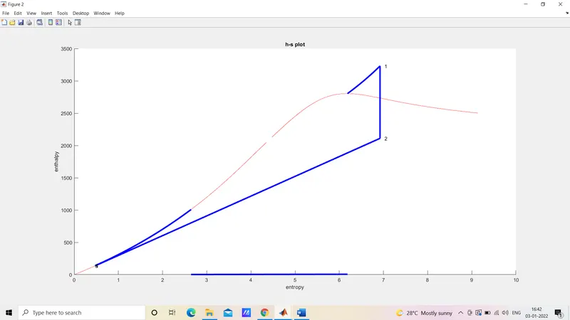
title('h-s plot')
xlabel('entropy')
ylabel('enthalpy')

Steps:

1. Start the program with 'clear all' 'close all' 'clc' command.
2. As our task is to take user input, to facilitate users to continue or end the program,we have introduced a while statement at the start of the script.
3. Now based on user inputs parameters 4 state points are calculated. Thermodynamic parameters include enthalpy H,entropy S , tehperature T , Pressure P and dryness faction X at state point 2. For calculating these parameters XSteam() i.e . steam table matlabprogram is required.
4. After calculating all parameters , the next objective is to calculate pump work ,turbine work, net work output, and thermal efficiency.
5. The next objective is to plot the graph for T_s and H_s.

RESULTS:

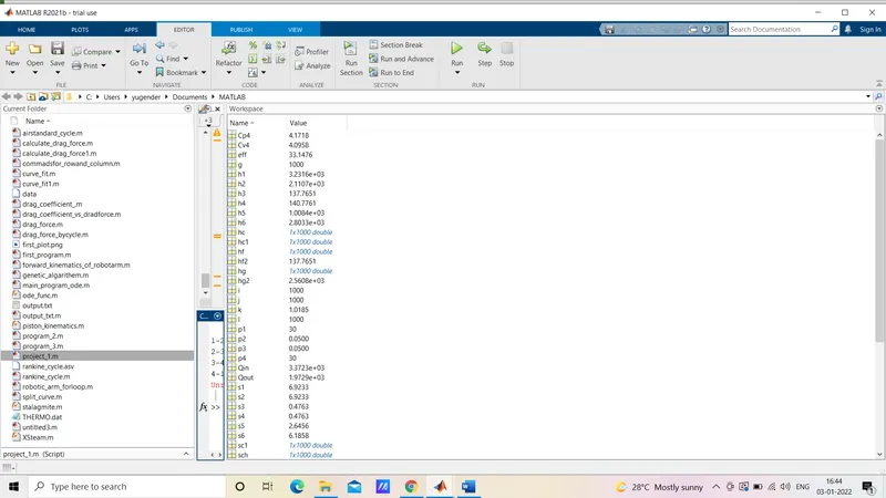
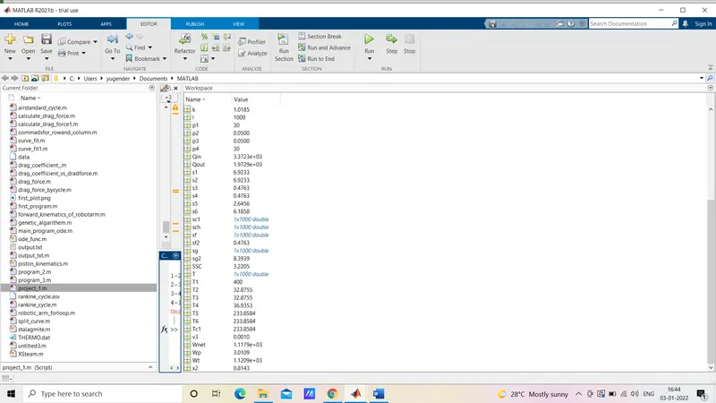
The calculated Net Work Output is Wnet = 1.117851878253914e+03

COMMAND WINDOW:

GRAPH:

T-S DIAGRAM

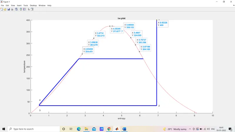
H-S DIAGRAM: