Rankine cycle Simulator using MATLAB

Objective: To create a Rankine cycle simulator using MATLAB

The rankine cycle as shown in the figure below, consists of the following processes:

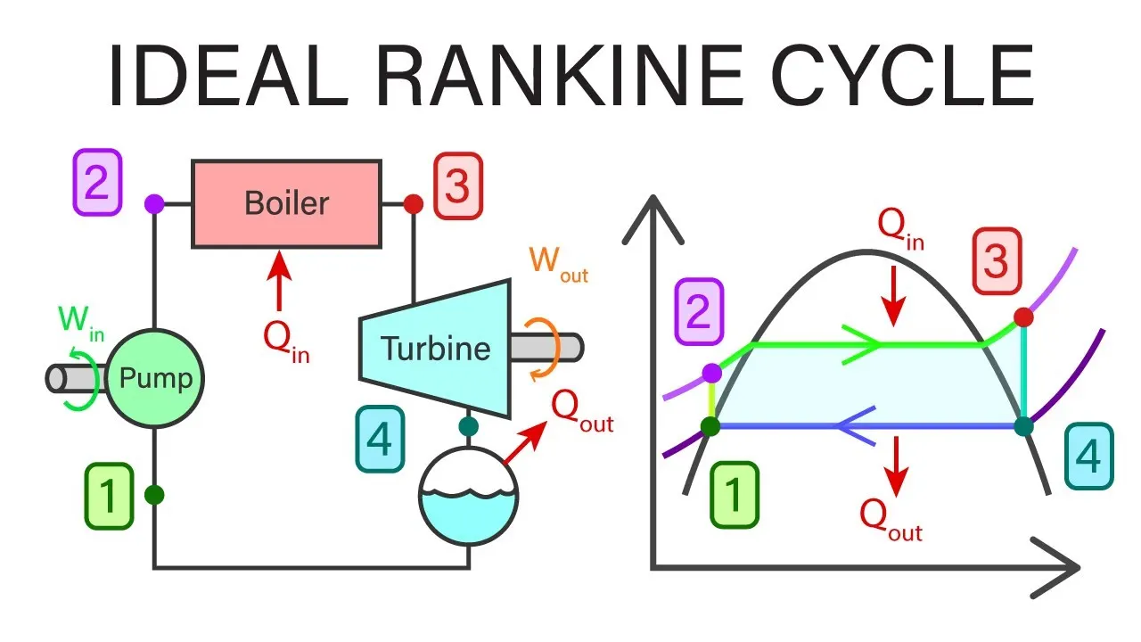
1-2: Isentropic compression in the pump

2-3: Constant pressure heat addition in the boiler

3-4: Isentropic expansion in the turbine

4-1: Constant pressure heat rejection in the condenser

The XSteam.m file contains properties of the water and steam such as enthalpy, entropy, specific volume,etc at different pressures and temperatures. Following is the method to extract these values from the file:

Xsteam('Tsat_p',40): Gives value of the saturation temperature at a given pressure (here 40 bar)

Xsteam('h_pT',40,300): Gives value of the enthalpy at a given pressure(here 40 bar) and temperature(here 300 C)

Xsteam('hL_p',40): Gives value of saturated liquid water at a given pressure (here 40 bar)

State points of the Rankine Cycle:

1: Inlet to the pump

2: Inlet to the boiler

a: Saturated liquid point of water at boiler pressure

b: Saturated vapour point of water at boiler pressure

3: Inlet point to the turbine

4: Turbine exit or condenser inlet

Inputs to the simulator:

Condenser pressure = 0.05 bar

Turbine Inlet temperature = 400 C

Boiler pressure = 30 bar

MATLAB code for the Rankine cycle simulator:

close all
clear all
clc

%Given data
p3 = 30;     %bar
p1=0.05;
t3=400;

p2=p3;
p4=p1;

%Entropies of state points
s1 = XSteam('sL_p',p1);
s2 = s1;
s3 = XSteam('s_pT',p3,t3);
s4 =s3;
sa = XSteam('sL_p',p2);
sb = XSteam('sV_p',p2);

%Temperatures of state points
t1 = XSteam('Tsat_p',p1);
t2= XSteam('T_ps',p2,s2);
t4 = t1;
ta = XSteam('T_ps',p2,sa);
tb = ta;

% specific volume at pump inlet
v1= XSteam('vL_p',p1);

% pump work (kJ/kg)
Wp = v1*(p2 - p1)*101.325;

%Enthapies  of state points
h1= XSteam('hL_p',p1);
h2 = h1 + Wp;
h3 = XSteam('h_pT',p3,t3);
h4 = XSteam('h_ps',p4,s4);
ha = XSteam('hL_p',p2);
hb = XSteam('hV_p',p2);

%Turbine work (kJ/kg)
Wt= h3-h4;

%Net work output (kJ/kg)
W = Wt - Wp;

%Back work ratio
BWR = Wt/Wp;


%entropy for process 2-a & b-3
Ta = linspace(t2,ta,100);
Tb = linspace(tb,t3,100);
for i=1:(length(Ta))
Sa(i) =  XSteam('s_pT',p2,Ta(i));
Sb(i) =  XSteam('s_pT',p2,Tb(i));
end

%Saturated liquid and vapour points calculation
P = linspace(0.001,230,1000);
for i = 1:length(P)
T(i) = XSteam('Tsat_p',P(i));
S_L(i) = XSteam('sL_p',P(i));
S_V(i) = XSteam('sV_p',P(i));
H_L(i) = XSteam('hL_p',P(i));
H_V(i) = XSteam('hV_p',P(i));
end

%Printing results
printf("At state point 1\n")
printf("P1 is : %d bar\n", p1)
printf("T1 is : %d bar\n", t1)
printf("H1 is : %d bar\n", h1)
printf("S1 is : %d bar\n\n", s1)

printf("At state point 2\n")
printf("P2 is : %d bar\n", p2)
printf("T2 is : %d bar\n", t2)
printf("H2 is : %d bar\n", h2)
printf("S2is : %d bar\n\n", s2)

printf("At state point 3\n")
printf("P3 is : %d bar\n", p3)
printf("T3 is : %d bar\n", t3)
printf("H3 is : %d bar\n", h3)
printf("S3 is : %d bar\n\n", s3)

printf("At state point 1\n")
printf("P4 is : %d bar\n", p4)
printf("T4 is : %d bar\n", t4)
printf("H4 is : %d bar\n", h4)
printf("S4 is : %d bar\n\n", s4)

printf("Wt is : %d kJ/kg\n", Wt)
printf("Wp is : %d kJ/kg\n", Wp)
printf("Wnet is : %d kJ/kg\n", W)
printf("Back work ratio is : %d", BWR)

%Plotting T-S diagram
figure(1)
hold on
plot(S_L,T,'color','b',S_V,T,'color','b')
plot(s1,t1,'.','markersize',15,'color','r')
plot(s2,t2,'.','markersize',15,'color','r')
line([s1 s2],[t1 t2],'linewidth',3,'color','b')
plot(sa,ta,'.','markersize',15,'color','r')
plot(Sa,Ta,'linewidth',3,'color','b');
plot(sb,tb,'.','markersize',15,'color','r')
line([sa sb],[ta tb],'linewidth',3,'color','b')
plot(Sb,Tb,'linewidth',3,'color','b');
plot(s3,t3,'.','markersize',15,'color','r')
plot(s4,t4,'.','markersize',15,'color','r')
line([s3 s4],[t3 t4],'linewidth',3,'color','b')
line([s4 s1],[t4 t1],'linewidth',3,'color','b')
title('Temperature-Entropy diagram')
xlabel('S (kJ/kg.C)')
ylabel('Temperature (K)')
grid on

%Plotting h-s diagram
figure(2)
hold on
plot(S_L,H_L,'color','b',S_V,H_V,'color','b')
plot(s1,h1,'.','markersize',15,'color','r')
plot(s2,h2,'.','markersize',15,'color','r')
line([s1 s2],[h1 h2],'linewidth',3,'color','b')
plot(s3,h3,'.','markersize',15,'color','r')
plot(s4,h4,'.','markersize',15,'color','r')
line([s2 s3],[h2 h3],'linewidth',3,'color','b')
line([s3 s4],[h3 h4],'linewidth',3,'color','b')
line([s4 s1],[h4 h1],'linewidth',3,'color','b')
title('Entahlpy-Entropy diagram')
xlabel('S (kJ/kg.C)')
ylabel('H (kJ/kg)')
grid on

Results:

State point properties:

T-S diagram:

Point 1 and 2 almost coincide with each other and can be if zoomed:

H-S Diagram: