Project 2 - Rankine cycle Simulator

OBJECTIVE:- Write a MATLAB code on Rankine Cycle Simulator and plot H-S & T-S diagrams.

PROBLEM STATEMENT:-

• Create a Rankine cycle simulator using MATLAB
• Our code should calculate the state points of the Rankine cycle based on user inputs.
• then plot the corresponding T-S & H-S plots for the given set of inputs. Title and axes labels are a must, while legends could be used if necessary.
• the presentation of our code will be taken into considerations while grading. Labeling section of our code using comments is appreciated
• Attach a report explaining the working of a Rankine cycle simulator and also research done by us.

Required inputs:

Turbine inlet temperature = 400 degrees Celcius

Turbine Inlet Pressure = 30 bars

Turbine outlet pressure = Condenser inlet pressure = 0.05 bars

Calculate the following-

• Net work output
• Back work ratio

THEORY & INTRODUCTION :-

The Rankine Cycle is one of many thermodynamic cycles that is used to produce mechanical work. This cycle in particular is used to predict the work produced by a steam turbine system in a heat engine. Heat engines are commenly found in things like trains and air conditioners.

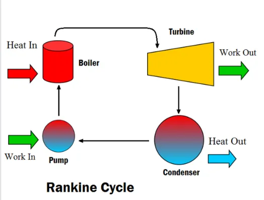
The Rankine cycle consist of four different components are-

1. Steam generator:- Turns the fluid at room temperature and pressure, to vapour or steam at an extremely high temperature, usually turned "Superheated Vapor".

2. Turbine:- The pressure is increase, resulting in a drop in temperature and producing mechanical work that leaves the system to be used.

3. Condenser:- Operates at a constant pressure where heat is released into the environment, compressing the state of the fluid back down to a liquid-gas mixture, that is mostly liquid. This state is otherwise known as "Saturated liquid".

4. Pump:- Pressurized the saturated liquid back up to the pressure of the turbine by bringing work back into the system, turning to a highly pressurized liquid which is usually referred to as a "Compressed Liquid".

Finally, the fluid goes back through the steam generator at constant pressure to return to superheated vapor.In order to easily analyse the Rankine Cycle, there are many idealization that engineers commenly make, so that the system can be understood in ideal situations. Additionally, there are some things throughout the cycle analysis that we will consider tobe 'ideal' meaning they work without any imperfections. Engineers tends to make these assumptions when analysing systems, in order to have an accurate representationof what is going on. But the fact is that nothing ever works out exactly how we expect or calculate and does not act the same way every time. This is especially true in the analysis of the Rankine Cycle. The reason that we say we are analysing a "Simple, Ideal Rankine Cycle" is because it is exactly that; simplified and ideal. In reality there are dozens of things that would have tobe accounted for to get an exact calculation, but they will be ignored for now in order to get a fundamental understanding of the cycle itself.

The concept and vocabulary needed to consider the system ideal are-

Adiabatic :- Does not loose heat

Isentropic :- Adiabatic and reversible or no change in entropy. Used when analysing the turbine and pump

Isobaric :- Constant pressure; considered when analysing the steam generator and condenser

Steady state :- the state of the fluid does not change with time

Steady flow :- that the mass of fluid flowing through the system is constant everywhere.

Boundary work :- Only consider changes that happens across the boundary of each component. There are other things that go on inside each component, but they are neglected for simplicity, since the final result would not be that different if they are included.

Compressed liquid :- A liquid that has been extremely pressurized

Pressure(P) :- One of the most important proparties, because it is usually given, allowing us to easily look up other proparty in our state Tables, and gives us an easy gage for where we are as we travel through the cycle.

Temperature(T) :- Is not always necessary to record but is used to give you of an idea of where you are in the cycle, and a gage that is easily understood. It is also listenin the state table, so it is sometimes useful to look up other proparties.

Entropy(S) :- An abstract concept used to represent the changes that occur to heat due to temperature.

Enthaly(h) :- Measure of the internal energy within a system. Each component analysed will be considered a 'system', allowing us to find an enthalpy value for each. This is essentially how the heat transfers through each of the components, and how we keep track of it's increase and decreases. Enthalpy is the proparty we will used to calculate work at the end according to the first law of thermodynamics.

Specific Volume (v):- Calcualted based on the volume of fluid per unit mass (different from total voume, which is unnecessary) and is used in this cycle to calculate the enthalpy out of the pump.

Quality(x) :- Measure of fluids liquid-gas mixture. If the fluid is in a superheated vapor state, or compressed liquid state it will not have a quality. Otherwise, it is a mixture of liquid and gas and the value will range from 0 to 1, 0 being a saturated liquid (still unpressurized but they close to the pressure limit) and 1 being a saturated vapor (steam, on the verge of being superheated).

Processes and Working :

There are four processes in the rankine cycle :

1. Process 1-2 : Isentropic Expansion in the turbine
2. Process 2-3 : Constant pressure Heat rejection in condenser
3. Process 3-4 : Isentropic compression in the pump
4. Process 4-1 : Constant pressure heat addition in the boiler

Rankine cycle efficiency ηR is -

Back Work Ratio:

The fraction of the work produced by the turbine is consumed by the compressor.

BW ratio=Wp/Wt

STEP BY STEP CODE EXPLANATION:-

1. First of all display all four points which are on the Rankine cycle(display command is used only for temporary reading and not save in memory).
2. described pressure and temperature values by user-defined.
3. find out the value of enthalpy(h1) and entropy(s1) from pressure and temperature from the XStream library in Matlab.
4. XStream library is nothing but the steam table, which is put in the same directory where the Matlab program is saved.
5. Find out all the points of inlet & outlet of turbine, condenser, pump, and boiler.
6. Also, find out the work done of pump and turbine
7. At state1 & 3 p3=p2 & p4=p1.
8. Find out net work done, heat supplied, heat rejected, efficiency & specific steam consumption.
9. finally, plot the H-S and T-S plots.
10. Link all the points i.e. 1-2-3-4-1.
11. gives the legend, title, label & label.
12. output the values of P, T, H, S for each state respectively.

% Rankine cycle simulator

clear all 
close all
clc

disp('RANKINE CYCLE SIMULATOR')
disp('1-2 is isentropic expansion in turbine')
disp('2-3 is constant pressure heat rejection in condenser')
disp('3-4 is isentropic compression in pump')
disp('4-1 is constant pressure heat addition in boiler')

p1 = input('enter the pressure at the inlet of turbine (in bar)=    ');
t1 = input('enter the temperature at the inlet of turbine (in degree celcius)=  ');
p2 = input('enter the pressure at the inlet of condenser (in bar)=  ');

%Steam condition at the inlet of turbine
h1 = XSteam('h_pt',p1,t1);
s1 = XSteam('s_pt',p1,t1);

% Steam condition at the outlet of turbine
sg2 = XSteam('sV_p',p2);
sf2 = XSteam('sL_p',p2);
sfg2 = sg2 - sf2;
x2 = (s1-sf2)/sfg2;
s2 = sf2 + x2*sfg2;

hf2 = XSteam('hL_p',p2);
hg2 = XSteam('hv_p',p2);
hfg2 = hg2 - hf2;
h2 = hf2 + x2*hfg2;

t2 = XSteam('Tsat_p',p2);

% Workdone by the turbine
W_T = h1-h2;

%Steam condition at the outlet of condenser
p3 = p2;
t3 = XSteam('Tsat_p',p2);
h3 = XSteam('hL_p',p2);
s3 = XSteam('sL_p',p2);
vf = XSteam('vL_p',p2);
t22 = t3;

% Calculation of pump work
W_P = vf*(p1-p2)*100;

% Steam condition at state-4
p4 = p1
h4 = W_P + h3;
s4 = s3;
t4 = XSteam('T_ph',p4,h4);

% Net workdone
W_net = W_T-W_P;

% Heat supplied
Q_s = h1-h4;

% Heat rejected
Q_r = h2-h3;

%Efficiency
efficiency = (W_net/Q_s);

% Specific steam consumption
SSC = 3600/W_net;

tf_sat = XSteam('Tsat_p',p1);
sf_sat = XSteam('sL_p',p1);
hf_sat = XSteam('hL_p',p1);
sg_sat = XSteam('sV_p',p1);
hg_sat = XSteam('hV_p',p1);

%Plotting T-S diagram
hold on

% for plotting saturation curve
tsat1 = linspace(0,374,1000);

for i = 1:length(tsat1)
    ss1(i) = XSteam('sL_T',tsat1(i));
end

for j = 1:length(tsat1)
    ss2(j) = XSteam('sV_T',tsat1(j));
end

plot(ss1,tsat1,'b')
plot(ss2,tsat1,'r')

% for saturation temperature at p1
temp = XSteam('Tsat_p',p1);
t = linspace(t4,temp,30);
for i = 1:length(t)
    S(i) = XSteam('s_pt',p1,t(i));
    hold on
end

t0 = linspace(temp,t1,300);
for i = 1:length(t0)
    s0(i) = XSteam('s_pt',p1,t0(i));
end

% for plotting turbine work
plot([s1 s2],[t1 t2],'g')

% for heat rejection in condenser
plot([s2 s3],[t2 t3],'b')

% for pump work
plot([s3 s4],[t3 t4],'r')

% plotting curve line (constant pressure line in wet region) from outlet of
% the pump to the point from where phase change starts
plot(S,t,'y')

% Plotting the phase change region
plot([sf_sat sg_sat],[tf_sat tf_sat],'y')

% Plotting the curved constant pressure line from where the phase change
% ends to the superheated point
plot(s0,t0,'y')

legend('Saturation Curve L','Saturation Curve V','Turbine','Condenser','Pump','Boiler','location','northwest')
title('T-S Diagram')
xlabel('Entropy')
ylabel('Temperature')

%plotting H-S diagram
figure(2)
hold on

% for plotting the saturation curve
tsat1 = linspace(0,374,1000);

for i = 1:length(tsat1)
    hh1(i) = XSteam('hL_T',tsat1(i));
end

for j = 1:length(tsat1)
    hh2(j) = XSteam('hV_T',tsat1(j));
end

plot(ss1,hh1,'b')
plot(ss2,hh2,'r')

%for plotting turbine
plot([s1 s2],[h1 h2],'g')

%for condenser
plot([s2 s3],[h2 h3],'b')

%for plotting pump
plot([s3 s4],[h3 h4],'r')
s = linspace(s3,s1,1000);

for i = 1:length(s)
    h(i) = XSteam('h_ps',p1,s(i));
end

%for plotting boiler
plot([s4 s1],[h4 h1],'y')
plot(s,h,'y')

legend('Saturation curve L','Saturation Curve V','Turbine','Condenser','Pump','Boiler','location','northwest')
title('H-S Diagram')
xlabel('Entropy')
ylabel('Enthalpy')

%Back work ratio
BWR = -(W_P/W_T);

%Output
%At state-1
fprintf('AT state point-1:rn')
fprintf('p1 is : %f Barrn',p1)
fprintf('T1 is : %f Deg Celciusrn',t1)
fprintf('H1 is : %f KJ/KGrn',h1)
fprintf('S1 is : %f KJ/KgKrn',s1)

%At state-2
fprintf('AT state point-2:rn')
fprintf('p2 is : %f Barrn',p2)
fprintf('T2 is : %f Deg Celciusrn',t2)
fprintf('H2 is : %f KJ/KGrn',h2)
fprintf('S2 is : %f KJ/KgKrn',s2)
fprintf('X is : %f rn',x2)

%At state-3
fprintf('AT state point-3:rn')
fprintf('p3 is : %f Barrn',p3)
fprintf('T3 is : %f Deg Celciusrn',t3)
fprintf('H3 is : %f KJ/KGrn',h3)
fprintf('S3 is : %f KJ/KgKrn',s3)

%At state-4
fprintf('AT state point-4:rn')
fprintf('p4 is : %f Barrn',p4)
fprintf('T4 is : %f Deg Celciusrn',t4)
fprintf('H4 is : %f KJ/KGrn',h4)
fprintf('S4 is : %f KJ/KgKrn',s4)

% Calculations
fprintf('Work done by Turbine : %f KJ/Kgrn',W_T)
fprintf('Work done by pump : %f KJ/Kgrn',W_P)
fprintf('Heat added in the boiler : %f KJ/Kgrn',Q_s)
fprintf('Heat rejected in the Condenser : %f KJ/Kgrn',Q_r)
fprintf('Thermal efficiency is : %f %%rn',efficiency*100)
fprintf('Species Steam Consumption : %f KJ/KWhrn',SSC)
fprintf('Back Work Ratio : %f  %%rn',BWR*100)

Result - The input, output screen, and the various state points with various parameters generated in the command window are shown below

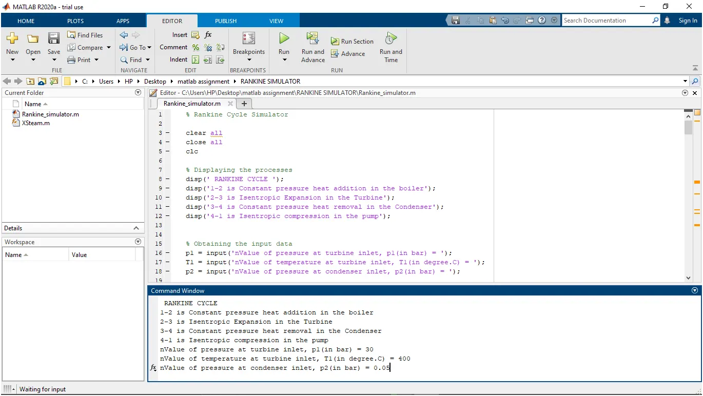
OUTPUT PLOTS:-

1) Temperature Vs Entropy plot :-

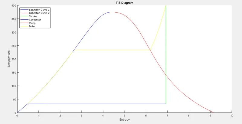
The above diagram shows the temperature vs entropy values. From points 1-2, as temperature increases, entropy also increases and vice versa. From points, 2-3 temperature remains constant but entropy increases continuously due to the turbine work as shown in the figure. Then temperature increases up to a critical point and then decreases at constant entropy and reducing temperature. From 4-1, the temperature remains constant at the low range and reaches the condenser through the pump.

From points, 3-4 temperature decreases because of the cooling effect through the heat exchanger i.e. fan. Here, the turbine gives positive work while the pump gives negative work, and according to that entropy increases and decreases respectively.

2) Enthalpy Vs Entropy plot:-

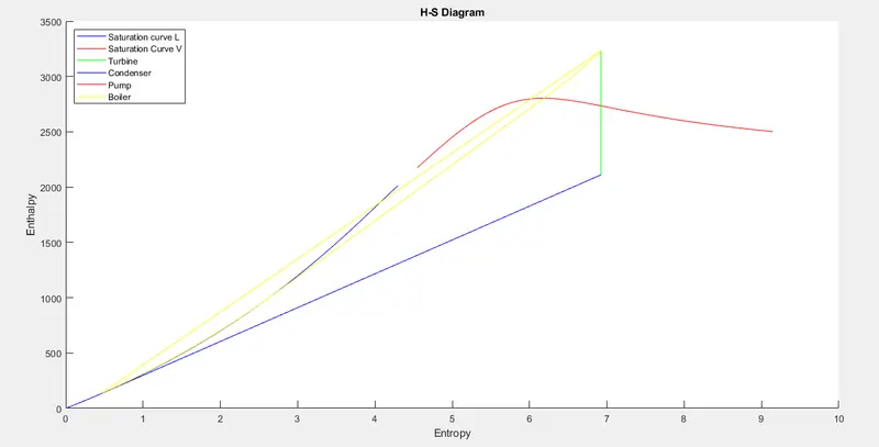
As we know that, entropy is directly proportional to the enthalpy, which is clearly proved from the above diagram. At a very small change of entropy, enthalpy changes widely as shown in the above figure. At the turbine, work is produced and that's why enthalpy increases at constant entropy, and thereafter this same cycle comes back with the same rate of change. The turbine produces work at constant entropy while the condenser produces work directly from entropy and enthalpy change. the rate of change of boiler is nearly same from start to end cycle.

OUTPUT SCREEN:-

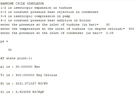
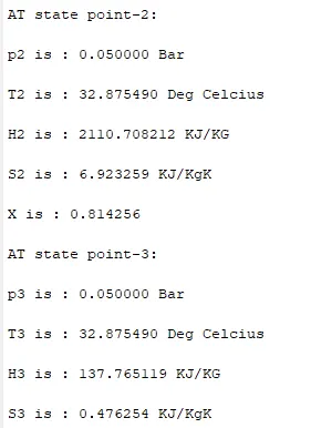
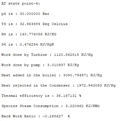
The above snapshots give all calculations related to the Rankine cycle at each point. Thermal efficiency is lower here because of pump work. As we know that pumps have different losses and due to this losses required more temperature. As temperature increases thermal efficiency also increases. Most of the heat is rejected from the condenser due to different cooling losses.

Back Work Ratio:-

The fraction of the work produced by the turbine is consumed by the pump.

Back Work Ratio for gas power cycle: 40% - 80%

Back Work Ratio for Vapor power cycle : 1% - 2%.

ERROR AND REMEDIES:-

1.

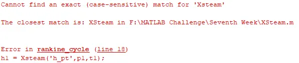
This error occurs due to the incorrect name of the saved file. As we know that, Matlab is case-sensitive, and if there have not matches a single word, it popup the error and thrown it in the command window. For rectifying this error we need to make confirm the written name in Matlab and file saving name in the same directory must be the same otherwise, it showing the same error.

2.

This error occurs due to the absence of parenthesis on either side. To solve this error we need to make confirm that, parenthesis must be on both the side. All the operators in Matlab must be in proper manner otherwise, it popup error in the command window. This is due to MATLAB is a scientific programming language and it works on matrices.

CONCLUSION:-

From the above plot and code, we can analyze the following points are-

1. When work is produced through the turbine and work consumed through a condenser, in both cases entropy changes but the temperature remains constant (from T-S diagram).
2. When fluid enters through the heat exchanger i.e. fan, only temperature decreases, entropy remains constant (from T-S diagram).
3. After turbine work temperature rises up to a critical point and then goes down.

In this way I write a detailed code in MATLAB, plot the T-S & H-S diagram as shown above. Also, I found some errors which are described above. Finally, I concluded some important points are described above.