Project 2 - Rankine cycle Simulator
Rankine cycle Simulator
Aim: To Write a code in MATLAB to Create a Rankine Cycle Simulator.
Introduction: RANKINE CYCLE: THE IDEAL CYCLE FOR VAPOR POWER CYCLES
Many of the impracticalities associated with the Carnot cycle can be eliminated by superheating the steam in the boiler and condensing it completely in the condenser, as shown schematically on a T-s diagram in Fig. 10–2. The cycle that results is the Rankine cycle, which is the ideal cycle for vapor power plants. The ideal Rankine cycle does not involve any internal irreversibilities and consists of the following four processes:
1-2 Isentropic compression in a pump
2-3 Constant pressure heat addition in a boiler
3-4 Isentropic expansion in a turbine
4-1 Constant pressure heat rejection in a condenser
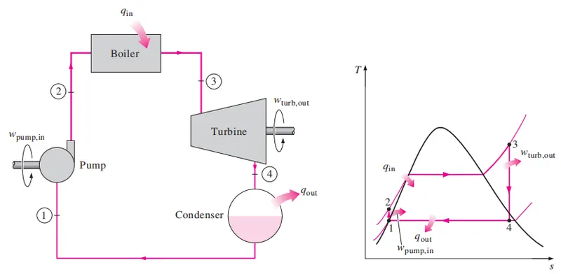
1-2 Isentropic compression in a pump: Water enters the pump at state 1 as saturated liquid and is compressed isentropically to the operating pressure of the boiler. The water temperature increases somewhat during this isentropic compression process due to a slight decrease in the specific volume of water. The vertical distance between states 1 and 2 on the T-s diagram is greatly exaggerated for clarity.
2-3 Constant pressure heat addition in a boiler: Water enters the boiler as a compressed liquid at state 2 and leaves as a superheated vapor at state 3. The boiler is basically a large heat exchanger where the heat originating from combustion gases, nuclear reactors, or other sources is transferred to the water essentially at constant pressure. The boiler, together with the section where the steam is superheated.
3-4 Isentropic expansion in a turbine: The superheated vapor at state 3 enters the turbine, where it expands isentropically and produces work by rotating the shaft connected to an electric generator. The pressure and the temperature of steam drop during this process to the values at state 4,
4-1 Constant pressure heat rejection in a condenser: where steam enters the condenser. At this state, steam is usually a saturated liquid–vapor mixture with a high quality. Steam is condensed at constant pressure in the condenser, which is basically a large heat exchanger, by rejecting heat to a cooling medium such as a lake, a river, or the atmosphere. Steam leaves the condenser as saturated liquid and enters the pump, completing the cycle. In areas where water is precious, the power plants are cooled by air instead of water. This method of cooling, which is also used in car engines, is called dry cooling.
Remembering that the area under the process curve on a T-s diagram represents the heat transfer for internally reversible processes, we see that the area under process curve 2-3 represents the heat transferred to the water in the boiler and the area under the process curve 4-1 represents the heat rejected in the condenser. The difference between these two (the area enclosed by the cycle curve) is the net work produced during the cycle.
Energy Analysis of the Ideal Rankine Cycle
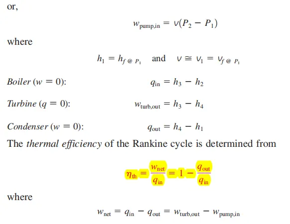
All four components associated with the Rankine cycle (the pump, boiler, turbine, and condenser) are steady-flow devices, and thus all four processes that make up the Rankine cycle can be analyzed as steady-flow processes. The kinetic and potential energy changes of the steam are usually small relative to the work and heat transfer terms and are therefore usually neglected. Then the steady-flow energy equation per unit mass of steam reduces to
h is specific enthalpy kJ/kg
(Qin - Qout) + (Win - Wout) =( he - hi) kJ/kg
The boiler and the condenser do not involve any work, and the pump and the turbine are assumed to be isentropic. Then the conservation of energy relation for each device can be expressed as follows:
Pump (q=0)
Wpump . h2 - h1
Required Inputs:
Turbine Inlet temperature = 400° C
Turbine Inlet Pressure = 30 bars
Turbine Outlet Pressure = 0.05 bars = Condenser Inlet Pressure
Code explanation
As per the question first print the rankine cycle. so using fprintf we can print in command window.
fprintf('\t \t \t Rankine Cycle Simulator \n ')
fprintf('******************************************************************')
fprintf('\n 1-2 Isentropic expansion in a turbine \n ')
fprintf('2-3 Constant pressure heat rejection in a condenser \n ')
fprintf('3-4 Isentropic compression in a pump \n ')
fprintf('4-1 Constant pressure heat addition in a boiler \n ')
fprintf('******************************************************************\n')
Terms used in the XSteam tabel.
% T Temperature (deg C)
% p Pressure (bar)
% h Enthalpy (kJ/kg)
% v Specific volume (m3/kg)
% rho Density
% s Specific entropy
% u Specific internal energy
% Cp Specific isobaric heat capacity
% Cv Specific isochoric heat capacity
% w Speed of sound
% my Viscosity
% tc Thermal Conductivity
% st Surface Tension
% x Vapour fraction
% vx Vapour Volume Fraction
% Given data as input
T1 = 400; % Turbine Inlet temperature in ° C
p1 = 30; % Turbine Inlet Pressure in bars
p2 = 0.05; %Turbine Outlet Pressure in bars = Condenser Inlet Pressure
% At state point 1 i e input to the turbine . whe have T1, p1 ve need h1 and s1 for T-s and h-s plots
% Reade data from Xsteam tabel.
%s_pT Specific entropy as a function of pressure and temperature (Returns saturated vapour entalpy if mixture.)
% The superheated vapor at state 1 enters the turbine, where it expands isentropically.
%The pressure and the temperature of steam drop during this process to the values at state 2,
s1 = XSteam('s_pT',p1,T1);
h1 = XSteam('h_pT',p1,T1);
fprintf('\n\t \t \t At state point 1 Turbine Inlet \n ')
fprintf('******************************************************************')
fprintf('\n Turbine Inlet temperature T1 is = %f ° C \n ',T1)
fprintf('Turbine Inlet Pressure p1 = %f bars \n ',p1)
fprintf('Specific entropy s1 = %f kj/kg-K \n ',s1)
fprintf('Entalpy h1 = %f kj/kg \n ',h1)
fprintf('******************************************************************\n')
% At state point 2 i e turbine outlet
% The superheated vapor at state 1 enters the turbine, where it expands isentropically and produces work by rotating the shaft connected to an electric
%The pressure and the temperature of steam drop during this process to the values at state 2,
s2 = s1; % because Isentropic expansion in a turbine where entropy is same
p2 = 0.05; %Turbine Outlet Pressure in bars = = Condenser Inlet Pressure
%T_ps Temperture as a function of pressure and entropy
T2 = XSteam('T_ps',p2,s2); %T2 can reade from tabel because we know s2 and p2 saturated temperature.
% To find h2
sf2 = XSteam('sL_p',p2); % Saturated liquid entropy at p2
sg2 = XSteam('sV_p',p2); %Saturated vapour entropy at p2
hf2 = XSteam('hL_p',p2); % Saturated liquid enthalpy at p2
hg2 = XSteam('hV_p',p2); % hV_p Saturated vapour enthalpy at p2
sfg2 = (sg2 - sf2); % sfg = (sg - sf)
hfg2 = (hg2 - hf2);
x = (s2 - sf2)/(sfg2);
h2 = hf2 + (x*hfg2); % Entalpy at p2
fprintf('\n\t \t \t At state point 2 Turbine outlet \n ')
fprintf('******************************************************************\n')
fprintf('Turbine outlet Pressure p2 = %f bars \n ',p2)
fprintf('Specific entropy s2 is = %f kj/kg-K \n ',s2)
fprintf('Turbine outlet temperature T2 is = %f ° C \n ',T2)
fprintf('Entalpy h2 is = %f kj/kg \n ',h2)
fprintf('******************************************************************\n')
% At state point 3 i e outlet of Condenser or inlet to pump
% Temperature and pressure is same which is equal to the state 3
T3 = T2; % Condenser Outlet Temperature
p3 = p2; % Condenser Outlet Pressure in bars = = pump Inlet Pressure
s3 = XSteam('sL_p',p3); % Saturated liquid entropy at p3
h3 = XSteam('hL_T',T3); %% Saturated liquid enthalpy at T3
fprintf('\n\t \t \t At state point 3 pump inlet or Condenser outlet \n ')
fprintf('******************************************************************\n')
fprintf('Condenser outlet Pressure p3 = %f bars \n ',p3)
fprintf('Condenser outlet temperature T2 is = %f ° C \n ',T3)
fprintf('Specific entropy s3 is = %f kj/kg-K \n ',s3)
fprintf('Entalpy h3 is = %f kj/kg \n ',h3)
fprintf('******************************************************************\n')
% variables for stage 4, 3-4 Isentropic compression in a pump
p4=p1; % Pressure out from the pump is equal to the pressure in to turbine
s4=s3; % Isentropic compression, constant entropy.
gama=1.4;
T4 = T3*(p4/p3)^((gama-1)/gama);
v3 = XSteam('vL_p',p3); %Specific volume at p3 (m3/kg)
Wp = v3*((p4-p3)*100); % Work done for the pump is kJ/kg
h4=h3+Wp; % W pump = h4-h3
fprintf('\n\t \t \t At state point 4 pump outlet or inlet to turbine \n ')
fprintf('******************************************************************\n')
fprintf('Pump outlet Pressure p4 = %f bars \n ',p4)
fprintf('Pump outlet temperature T2 = %f ° C \n ',T4)
fprintf('Specific entropy s4 = %f kj/kg-K \n ',s4)
fprintf('Entalpy h4 = %f kj/kg \n ',h4)
fprintf('******************************************************************\n')
p5=p1; %Pressure out from the pump is equal to the pressure in to turbine
T5 = XSteam('Tsat_p',p5); % Temp at p5
s5 = XSteam('sL_p',p5); % entropy at p5
h5 = XSteam('hL_T',T5); % enthalpy at T5
% variables for stage 5
fprintf('\n\t \t \t At state point 5 \n ')
fprintf('******************************************************************\n')
fprintf('p5 = %f bars \n ',p5)
fprintf('T5 = %f ° C \n ',T5)
fprintf('s5 = %f kj/kg-K \n ',s5)
fprintf('h5 = %f kj/kg \n ',h5)
fprintf('******************************************************************\n')
% variables for stage 6
% p6, s6 and h6 at T6
T6=T5;
p6=XSteam('psat_T',T6);
s6=XSteam('sV_T',T6);
h6=XSteam('hV_T',T6);
fprintf('\n\t \t \t At state point 6 \n ')
fprintf('******************************************************************\n')
fprintf('p6 = %f bars \n ',p6)
fprintf('T6 = %f ° C \n ',T6)
fprintf('s6 = %f kj/kg-K \n ',s6)
fprintf('h6 = %f kj/kg \n ',h6)
fprintf('******************************************************************\n')
% Calculations for turbine and pump.
% Pump work Wp = v3*((p4-p3)*100); % Work done by pump is kJ/kg
fprintf('Work for the pump is Wp_in = %f kJ/kg \n ',Wp);
% Tubrine work
% Work done by the turbine is Wt_out kJ/kg
Wt=h1-h2;
fprintf('Work by the turbine is Wt_out = %f kJ/kg \n ',Wt);
% Met work is given Wnet = Wt - Wp
Wnet=Wt-Wp;
fprintf('Net work is Wnet = %f kJ/kg \n ',Wnet)
% heat added to the boiler Qin is Qin=h1-h4;
Qin=h1-h4;
% Heat removed by Condenser is Qout is Qout=h2-h3;
Qout=h2-h3;
% Thermal efficiency of rankine cycle is
Nth=Wnet/Qin;
fprintf('Thermal efficiency of rankine cycle is Nth = %f kJ/kg \n ',Nth)
%specific steam consumption is given by 3600/network kg/kWh
SSC = 3600/Wnet;
fprintf('specific steam consumption of rankine cycle is SSC = %f kJ/kg \n ',SSC)
% To plot T-s and h-s we need data points for every change of s and h wrt temperature
% For Specific entropy S for liquid Wrt temperature
T = linspace(0,400,750);
for i = 1:length(T)
S_L(i) = XSteam('sL_T',T(i)); % entropy of Liquid state for every temperature
end
% For Specific entropy S for vapour stae Wrt temperature
for j = 1:length(T)
S_V(j) = XSteam('sV_T',T(j)); % entropy of Liquid state for every temperature
end
% For h Enthalpy
% h Enthalpy at Liquid state for every temperature
for k = 1: length(T)
H_L(k) = XSteam('hL_T',T(k));
end
% h Enthalpy at Liquid state for every temperature
for l = 1: length(T)
H_V(l) = XSteam('hV_T',T(l));
end
% PLOTS
% Plot T - s
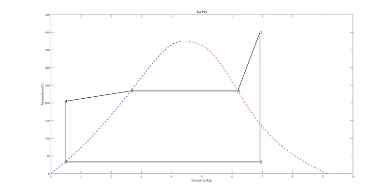
figure(1) % for T-s
plot(S_L,T,'--','color','b','linewidth',1.5)
hold on
plot(S_V,T,'--','color','r','linewidth',1.5)
plot([s1 s2 s3 s4 s5 s6 s1],[T1 T2 T3 T4 T5 T6 T1],'linewidth',1.5,'color','k')
plot(s1,T1,'*', 'color','y');
plot(s2,T2,'*', 'color','y');
plot(s3,T3,'*', 'color','y');
plot(s4,T4,'*', 'color','y');
plot(s5,T5,'*', 'color','y');
plot(s6,T6,'*', 'color','y');
text(s1,T1,'1','FontSize',14);
text(s2,T2,'2','FontSize',14);
text(s3,T3,'3','FontSize',14);
text(s4,T4,'4','FontSize',14);
text(s5,T5,'5','FontSize',14);
text(s6,T6,'6','FontSize',14);
title('h-s Plot')
axis([0 10 0 450])
xlabel('Entropy [kJ/kg] ')
ylabel('Temperature [°C]')
% Plot h -s
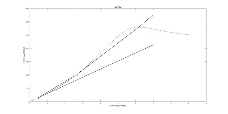
figure(2)
plot(S_L,H_L,'--','color','b','linewidth',1.5)
hold on
plot(S_V,H_V,'--','color','r','linewidth',1.5)
plot([s1 s2 s3 s4 s5 s6 s1],[h1 h2 h3 h4 h5 h6 h1],'linewidth',1.5,'color','k')
plot(s1,h1,'*', 'color','y');
plot(s2,h2,'*', 'color','y');
plot(s3,h3,'*', 'color','y');
plot(s4,h4,'*', 'color','y');
plot(s5,h5,'*', 'color','y');
plot(s6,h6,'*', 'color','y');
text(s1,h1,'1','FontSize',14);
text(s2,h2,'2','FontSize',14);
text(s3,h3,'3','FontSize',14);
text(s4,h4,'4','FontSize',14);
text(s5,h5,'5','FontSize',14);
text(s6,h6,'6','FontSize',14);
title('s-h Plot')
xlabel('s (Entropy) [KJ/KgK]')
ylabel('h (Enthalpy) [KJ/Kg]')
Program:
% Write a code in MATLAB to Create a Rankine Cycle Simulator.
close all
clear all
clc

fprintf('\t \t \t Rankine Cycle Simulator \n  ')
fprintf('******************************************************************')
fprintf('\n 1-2 Isentropic expansion in a turbine \n ')
fprintf('2-3 Constant pressure heat rejection in a condenser \n ')
fprintf('3-4 Isentropic compression in a pump \n ')
fprintf('4-1 Constant pressure heat addition in a boiler \n ')
fprintf('******************************************************************\n')

% T     Temperature (deg C)
% p	    Pressure    (bar)
% h	    Enthalpy    (kJ/kg)
% v	    Specific volume (m3/kg)
% rho	Density
% s	    Specific entropy
% u	    Specific internal energy
% Cp	Specific isobaric heat capacity
% Cv	Specific isochoric heat capacity
% w	    Speed of sound
% my	Viscosity
% tc	Thermal Conductivity
% st	Surface Tension
% x	    Vapour fraction
% vx	Vapour Volume Fraction

% Given data as input
T1 = 400; % Turbine Inlet temperature in ° C
p1 = 30;  % Turbine Inlet Pressure in bars
p2 = 0.05; %Turbine Outlet Pressure in  bars =  = Condenser Inlet Pressure

% At state point 1 i e input to the turbine . whe have T1, p1 ve need h1 and s1 for T-s and h-s plots
% Reade data from Xsteam tabel.
%s_pT	Specific entropy as a function of pressure and temperature (Returns saturated vapour entalpy if mixture.)
% The superheated vapor at state 1 enters the turbine, where it expands isentropically.
%The pressure and the temperature of steam drop during this process to the values at state 2,

s1 = XSteam('s_pT',p1,T1);
h1 = XSteam('h_pT',p1,T1);

fprintf('\n\t \t \t At state point 1 Turbine Inlet  \n ')
fprintf('******************************************************************')
fprintf('\n Turbine Inlet temperature T1 is = %f ° C \n ',T1)
fprintf('Turbine Inlet Pressure p1 = %f bars \n ',p1)
fprintf('Specific entropy s1 = %f kj/kg-K \n ',s1)
fprintf('Entalpy  h1 =  %f kj/kg \n ',h1)
fprintf('******************************************************************\n')


% At state point 2 i e turbine outlet
% The superheated vapor at state 1 enters the turbine, where it expands isentropically and produces work by rotating the shaft connected to an electric
%The pressure and the temperature of steam drop during this process to the values at state 2,
s2 = s1; % because Isentropic expansion in a turbine where entropy is same
p2 = 0.05;  %Turbine Outlet Pressure in  bars =  = Condenser Inlet Pressure
%T_ps	Temperture as a function of pressure and entropy
T2 = XSteam('T_ps',p2,s2); %T2 can reade from tabel because we know s2 and p2 saturated temperature.

% To find h2
sf2 = XSteam('sL_p',p2); % Saturated liquid entropy at p2
sg2 = XSteam('sV_p',p2); %Saturated vapour entropy at p2
hf2 = XSteam('hL_p',p2); % Saturated liquid enthalpy at p2
hg2 = XSteam('hV_p',p2); % hV_p	Saturated vapour enthalpy at p2
sfg2 = (sg2 - sf2);      % sfg = (sg - sf)
hfg2 = (hg2 - hf2);
x = (s2 - sf2)/(sfg2);
h2 = hf2 + (x*hfg2);    % Entalpy at p2

fprintf('\n\t \t \t At state point 2 Turbine outlet  \n ')
fprintf('******************************************************************\n')
fprintf('Turbine outlet Pressure p2 = %f bars \n ',p2)
fprintf('Specific entropy s2 is = %f kj/kg-K \n ',s2)
fprintf('Turbine outlet temperature T2 is = %f ° C \n ',T2)
fprintf('Entalpy  h2  is = %f kj/kg \n ',h2)
fprintf('******************************************************************\n')

% At state point 3 i e  outlet of Condenser or inlet to pump
% Temperature and pressure is same which is equal to the state 3
T3 = T2;                %  Condenser  Outlet Temperature
p3 = p2;                % Condenser  Outlet Pressure in  bars =  = pump Inlet Pressure
s3 = XSteam('sL_p',p3);  % Saturated liquid entropy at p3
h3 = XSteam('hL_T',T3);  %% Saturated liquid enthalpy at T3

fprintf('\n\t \t \t At state point 3 pump inlet or Condenser outlet  \n ')
fprintf('******************************************************************\n')
fprintf('Condenser outlet Pressure p3 = %f bars \n ',p3)
fprintf('Condenser outlet temperature T2 is = %f ° C \n ',T3)
fprintf('Specific entropy s3 is = %f kj/kg-K \n ',s3)
fprintf('Entalpy  h3 is = %f kj/kg \n ',h3)
fprintf('******************************************************************\n')


% variables for stage 4, 3-4 Isentropic compression in a pump
p4=p1;   % Pressure out from the pump is equal to the pressure in to turbine
s4=s3;   % Isentropic compression, constant entropy.

gama=1.4;

T4 = T3*(p4/p3)^((gama-1)/gama);
v3 = XSteam('vL_p',p3);   %Specific volume at p3 (m3/kg)
Wp = v3*((p4-p3)*100);    % Work done for the  pump is kJ/kg
h4=h3+Wp;                 % W pump = h4-h3


fprintf('\n\t \t \t At state point 4 pump outlet or inlet to turbine  \n ')
fprintf('******************************************************************\n')
fprintf('Pump outlet Pressure p4 = %f bars \n ',p4)
fprintf('Pump outlet temperature T2 = %f ° C \n ',T4)
fprintf('Specific entropy s4 = %f kj/kg-K \n ',s4)
fprintf('Entalpy  h4 =  %f kj/kg \n ',h4)
fprintf('******************************************************************\n')

p5=p1;    %Pressure out from the pump is equal to the pressure in to turbine
T5 = XSteam('Tsat_p',p5);  % Temp at p5
s5 = XSteam('sL_p',p5);   % entropy at p5
h5 = XSteam('hL_T',T5);   %  enthalpy at T5

% variables for stage 5
fprintf('\n\t \t \t At state point 5  \n ')
fprintf('******************************************************************\n')
fprintf('p5 = %f bars \n ',p5)
fprintf('T5 = %f ° C \n ',T5)
fprintf('s5 = %f kj/kg-K \n ',s5)
fprintf('h5 =  %f kj/kg \n ',h5)
fprintf('******************************************************************\n')

% variables for stage 6
% p6, s6 and h6 at T6
T6=T5;
p6=XSteam('psat_T',T6);
s6=XSteam('sV_T',T6);
h6=XSteam('hV_T',T6);

fprintf('\n\t \t \t At state point 6  \n ')
fprintf('******************************************************************\n')
fprintf('p6 = %f bars \n ',p6)
fprintf('T6 = %f ° C \n ',T6)
fprintf('s6 = %f kj/kg-K \n ',s6)
fprintf('h6 =  %f kj/kg \n ',h6)
fprintf('******************************************************************\n')

% Calculations for turbine and pump.
% Pump work Wp = v3*((p4-p3)*100);    % Work done by pump is kJ/kg

fprintf('Work for the pump is Wp_in = %f kJ/kg \n ',Wp);

% Tubrine work
% Work done by the turbine is Wt_out kJ/kg
Wt=h1-h2;
fprintf('Work by the turbine is Wt_out = %f kJ/kg \n ',Wt);

% Met work is given Wnet = Wt - Wp
Wnet=Wt-Wp;
fprintf('Net work is Wnet = %f kJ/kg \n ',Wnet)

% heat added to the boiler Qin is Qin=h1-h4;
Qin=h1-h4;
% Heat removed by Condenser is Qout is Qout=h2-h3;
Qout=h2-h3;

% Thermal efficiency of rankine cycle is
Nth=Wnet/Qin;
fprintf('Thermal efficiency of rankine cycle is  Nth = %f kJ/kg \n ',Nth)

%specific steam consumption is given by 3600/network kg/kWh

SSC = 3600/Wnet;

fprintf('specific steam consumption of rankine cycle is  SSC = %f kJ/kg \n ',SSC)


% To plot T-s and h-s we need data points for every change of s and h wrt temperature

% For Specific entropy S for liquid  Wrt temperature
T = linspace(0,400,750);
for i = 1:length(T)
    S_L(i) = XSteam('sL_T',T(i)); % entropy of Liquid state for every temperature
end

% For Specific entropy S for vapour stae  Wrt temperature

for j = 1:length(T)
    S_V(j) = XSteam('sV_T',T(j)); % entropy of Liquid state for every temperature
end

% For h	 Enthalpy
% h Enthalpy at Liquid state for every temperature

for k = 1: length(T)
    H_L(k) = XSteam('hL_T',T(k));
end


% h Enthalpy at Liquid state for every temperature

for l = 1: length(T)
    H_V(l) = XSteam('hV_T',T(l));
end


% PLOTS

% Plot T - s
figure(1)    % for T-s

plot(S_L,T,'--','color','b','linewidth',1.5)
hold on
plot(S_V,T,'--','color','r','linewidth',1.5)

plot([s1 s2 s3 s4 s5 s6 s1],[T1 T2 T3 T4 T5 T6 T1],'linewidth',1.5,'color','k')

plot(s1,T1,'*', 'color','y');
plot(s2,T2,'*', 'color','y');
plot(s3,T3,'*', 'color','y');
plot(s4,T4,'*', 'color','y');
plot(s5,T5,'*', 'color','y');
plot(s6,T6,'*', 'color','y');

text(s1,T1,'1','FontSize',14);
text(s2,T2,'2','FontSize',14);
text(s3,T3,'3','FontSize',14);
text(s4,T4,'4','FontSize',14);
text(s5,T5,'5','FontSize',14);
text(s6,T6,'6','FontSize',14);
title('h-s Plot')
axis([0 10 0 450])
xlabel('Entropy [kJ/kg] ')
ylabel('Temperature [°C]')

% Plot  h -s


figure(2)
plot(S_L,H_L,'--','color','b','linewidth',1.5)
hold on
plot(S_V,H_V,'--','color','r','linewidth',1.5)


plot([s1 s2 s3 s4 s5 s6 s1],[h1 h2 h3 h4 h5 h6 h1],'linewidth',1.5,'color','k')
plot(s1,h1,'*', 'color','y');
plot(s2,h2,'*', 'color','y');
plot(s3,h3,'*', 'color','y');
plot(s4,h4,'*', 'color','y');
plot(s5,h5,'*', 'color','y');
plot(s6,h6,'*', 'color','y');


text(s1,h1,'1','FontSize',14);
text(s2,h2,'2','FontSize',14);
text(s3,h3,'3','FontSize',14);
text(s4,h4,'4','FontSize',14);
text(s5,h5,'5','FontSize',14);
text(s6,h6,'6','FontSize',14);

title('s-h Plot')
xlabel('s (Entropy) [KJ/KgK]')
ylabel('h (Enthalpy) [KJ/Kg]')
Results: Write a code in MATLAB to Create a Rankine Cycle Simulator is done
1. Plots for T-s and h-s are obtained as per the ideal cycle of Rankine.