Project 2 - Rankine cycle Simulator
AIM:
To devolop a matlab program to simulate the Rankine cycle from the XSteam library and to calculate the thermal efficiency and plot the T-S and H-S diagram for the same.
DEFINITION:
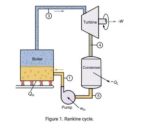
The Rankine cycle is a model used to predict the performance of steam turbine systems. The Rankine cycle is an idealized thermodynamic cycle of a heat engine that converts heat into mechanical work while undergoing a phase change. It is an idealized cycle in which friction losses in each of the four components are neglected. The heat is supplied externally to a closed loop, which usually uses water as the working fluid.
RANKINE CYCLE PROCESS
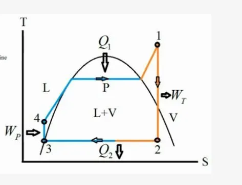
1-2-3 process-> Isobaric Heat Transfer. High pressure liquid enters the boiler from the feed pump (1) and is heated to the saturation temperature (2). Further addition of energy causes evaporation of the liquid until it is fully converted to saturated steam (3).
3-4 process- ->Isentropic Expansion. The vapor is expanded in the turbine, thus producing work which may be converted to electricity. In practice, the expansion is limited by the temperature of the cooling medium and by the erosion of the turbine blades by liquid entrainment in the vapor stream as the process moves further into the two-phase region. Exit vapor qualities should be greater than 90%.
4-5 process- -> Isobaric Heat Rejection. The vapor-liquid mixture leaving the turbine (4) is condensed at low pressure, usually in a surface condenser using cooling water. In well designed and maintained condensers, the pressure of the vapor is well below atmospheric pressure, approaching the saturation pressure of the operating fluid at the cooling water temperature.
5-1 process- ->Isentropic Compression. The pressure of the condensate is raised in the feed pump. Because of the low specific volume of liquids, the pump work is relatively small and often neglected in thermodynamic calculations.
MATLAB CODE:
clear all
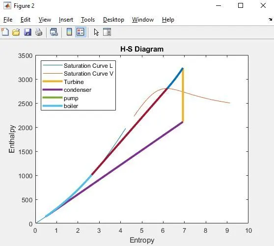
close all
clc

fprintf('Rankine cycle\n')
fprintf('1-2 is Isentropic Expansion in the Turbine\n')
fprintf('2-3 is constant pressure Heat Rejection by the Condensor\n')
fprintf('3-4 is Isentropic Compression in the Pump\n')
fprintf('4-1 is the Constant Pressure Heat Addition by the Boiler\n')

% Given values - P1,T1,P2
Inlet_pressure = input('Enter the Pressure at the Turbine inlet(in bar):')
Inlet_temp = input('Enter the Temperature at the Turbine inlet(in Degree Celcius):')
Outlet_pressure = input('Enter the Pressure at the Condenser:')


h1 = XSteam('h_pT',Inlet_pressure,Inlet_temp);
s1 = XSteam('s_pT',Inlet_pressure,Inlet_temp);

fprintf('At state point 1:\n')
fprintf('P1 is: %d\n',Inlet_pressure)
fprintf('T1 is: %f\n',Inlet_temp)
fprintf('H1 is: %f\n',h1)
fprintf('S1 is: %f\n\n',s1)

% State point-2
s2 = s1;
t2 = XSteam('T_ps',Outlet_pressure,s2);

sf = XSteam('sL_T',t2);
sg = XSteam('sV_T',t2);
sfg = sg-sf;

%Dryness fraction
x = (s2-sf)/sfg;

hf = XSteam('hL_T',t2);
hg = XSteam('hV_T',t2);
hfg = hg-hf;

h2 = hf+(x*hfg);

fprintf('At state point 2:\n')
fprintf('P2 is: %f\n',Outlet_pressure)
fprintf('T2 is: %f\n',t2)
fprintf('H2 is: %f\n',h2)
fprintf('S2 is: %f\n',s2)
fprintf('X2 is: %f\n\n',x)

% State point 3

p3 = Outlet_pressure;

t3 = XSteam('Tsat_p',p3);

s3 = XSteam('sL_p',p3);

h3 = XSteam('hL_p',p3);

fprintf('At state point 3:\n')
fprintf('P3 is: %f\n',p3)
fprintf('T3 is: %f\n',t3)
fprintf('H3 is: %f\n',h3)
fprintf('S3 is: %f\n\n',s3)

% State point 4

p4 = Inlet_pressure;

s4 = s3;

h4 = XSteam('h_ps',p4,s4);

t4 = XSteam('T_ps',p4,s4);
%T2 = Inlet_temp*(Outlet_pressure/Inlet_pressure)^(0.4/1.4)

fprintf('At state point 4:\n')
fprintf('P4 is: %f\n',p4)
fprintf('T4 is: %f\n',t4)
fprintf('H4 is: %f\n',h4)
fprintf('S4 is: %f\n\n',s4)

% State point 5

p5 = p4;

t5 = XSteam('Tsat_p',p5);

s5 = XSteam('sL_p',p5);

h5 = XSteam('hL_p',p5);

fprintf('At state point 5:\n')
fprintf('P5 is: %f\n',p5)
fprintf('T5 is: %f\n',t5)
fprintf('H5 is: %f\n',h5)
fprintf('S5 is: %f\n\n',s5)

% State point 6

p6 = p4;

t6 = XSteam('Tsat_p',p6);

s6 = XSteam('sV_p',p6);

h6 = XSteam('hV_p',p6);

fprintf('At state point 6:\n')
fprintf('P6 is: %f\n',p6)
fprintf('T6 is: %f\n',t6)
fprintf('H6 is: %f\n',h6)
fprintf('S6 is: %f\n\n',s6)

% Turbine work
Wt = h1-h2;

% Pump work
Wp = h4-h3;

% total net work
Wnet = Wt-Wp;

Qin = h1-h4;

% Thermal efficiency
Ntherm = Wnet/Qin;

% Specific Steam Consumption
SSE = 3600/Wnet;

fprintf('Wt is: %f\n',Wt)
fprintf('Wp is: %f\n',Wp)
fprintf('Wnet is: %f\n',Wnet)
fprintf('Ntherm is: %f\n',Ntherm)
fprintf('S.S.E is: %f\n',SSE)

%plotting saturation curve for T-S diagram

figure(1)

T1 = linspace(1,373,1000);
for i=1:length(T1)

    sf(i) = XSteam('sL_T',T1(i));
    sg(i) = XSteam('sV_T',T1(i));
    hf(i) = XSteam('hL_T',T1(i));
    hg(i) = XSteam('hV_T',T1(i));
end
plot(sf,T1)
hold on
plot(sg,T1)

%Plotting T-S diagram

hold on
plot([s1 s2],[Inlet_temp t2],'linewidth',3)
plot([s2 s3],[t2 t3],'linewidth',3)
plot([s3 s4],[t3 t4],'linewidth',3)

tc1 = linspace(t4,t5,1000);
pc1 = linspace(p4,p5,1000);
for i=1:length(tc1)
    sc1(i) = XSteam('s_pT',pc1(i),tc1(i));
end
plot(sc1,tc1,'linewidth',3)
plot([s5 s6],[t5 t6],'linewidth',3)
tc2 = linspace(t6,Inlet_temp,1000);
pc2 = linspace(p6,Inlet_pressure,1000);
for i=1:length(tc2)
    sc2(i) = XSteam('s_pT',pc2(i),tc2(i));
end
plot(sc2,tc2,'linewidth',3)
xlabel('Entropy(S)')
ylabel('Temperature(T)')
legend('Saturation Curve L','Saturation Curve V','Turbine','condenser','pump','boiler','location','northwest')
title('T-S Diagram')

% Saturation curve for H-S Diagram
figure(2)
T2 = linspace(1,373,1000);
for j=1:length(T2)

    sf(j) = XSteam('sL_T',T2(j));
    sg(j) = XSteam('sV_T',T2(j));
    hf(j) = XSteam('hL_T',T2(j));
    hg(j) = XSteam('hV_T',T2(j));
end
plot(sf,hf)
hold on
plot(sg,hg)

%Plotting H-S diagram:

hold on
plot([s1 s2],[h1 h2],'linewidth',3)
hc1 = linspace(h2,h3,1000);
pc3 = linspace(Outlet_pressure,p3,1000);
for i=1:length(hc1)
    sc3(i) = XSteam('s_ph',pc3(i),hc1(i));
end
plot(sc3,hc1,'linewidth',3)
plot([s3 s4],[h3 h4],'linewidth',3)
hc2 = linspace(h4,h5,1000);
pc4 = linspace(p4,p5,1000);
for i=1:length(hc2)
    sc4(i) = XSteam('s_ph',pc4(i),hc2(i));
end
plot(sc4,hc2,'linewidth',3)
hc3 = linspace(h5,h6,1000);
pc5 = linspace(p5,p6,1000);
for i=1:length(hc3)
    sc5(i) = XSteam('s_ph',pc5(i),hc3(i));
end
plot(sc5,hc3,'linewidth',3)
hc4 = linspace(h6,h1,1000);
pc6 = linspace(p6,Inlet_pressure,1000);
for i=1:length(hc4)
    sc6(i) = XSteam('s_ph',pc6(i),hc4(i));
end
plot(sc6,hc4,'linewidth',3)
hold on
xlabel('Entropy')
ylabel('Enthalpy')
legend('Saturation Curve L','Saturation Curve V','Turbine','condenser','pump','boiler','location','northwest')
title('H-S Diagram')
1. The given values for the current simulation are inlet pressure and temperature and the Outlet pressure ie. P2 with values 30, 400 and 0.05 respectivily.
2. XSteam functions are the matlab code for steam table which helps to input the values for saturated, superheated regions as well it can be defined with respect to any two variables like pressure,temperature,entropy,enthalpy etc.
XSteam take 2 or 3 arguments. The first argument must always be the steam table function you want to use. The other arguments are the inputs to that function.
h1 = XSteam('h_pT',Inlet_pressure,Inlet_temp);
s1 = XSteam('s_pT',Inlet_pressure,Inlet_temp);
The above syntax defines the value of enthalpy at a purticular point w.r.t the pressure and temperature and the second syntax will give the value of entropy with pressure and temperature as the inputs to that function.
3. At state point #2
s2 = s1; #As per the curve the entropy at point 1 is equal to entropy at point 2
t2 = XSteam('T_ps',Outlet_pressure,s2); # Xsteam function is used to find the value of T2 with pressure and entropy as the inputs
sf = XSteam('sL_T',t2); # Specific Entropy at liquid state
sg = XSteam('sV_T',t2); # Specific Entropy at vapour state
sfg = sg-sf; # Sfg= Difference in Specific Entropy at the above two conditions
4. x = (s2-sf)/sfg;
hf = XSteam('hL_T',t2); # Specific enthalpy at liquid state
hg = XSteam('hV_T',t2); # Specific enthalpy at vapour state
hfg = hg-hf; # Hfg= Difference in Specific enthalpy at the above two conditions
x is defined as the dryness fraction which is ratio of the mass of actual dry steam to the mass of steam containing it. It is usually expressed by the symbol ‘x’ .
5. At state point 3, the pressure at this point is equal to P2 ie the outlet pressure, as the pressure is constant during this process. The rest of the values are calculated using the Xsteam table.
6. p4 = Inlet_pressure; # From p4 to p1, the pressure inside the boiler will be constant,as it undergoes reversible adiabatic process.
s4 = s3; # As per the plot, we know entropy at point 3 is equal to the entropy at point 4
h4 = XSteam('h_ps',p4,s4);
t4 = XSteam('T_ps',p4,s4);
7. Similarly at state point 5 and 6, the pressure will be same as that of pressure at point 4. The rest of the values can be established from the Xsteam table.
8. After all the processes are completed, as per the given question, additional parameters have to be inputted which are given below:
% Turbine work in 1->2 process
Wt = h1-h2;
% Pump work in 3->4 process
Wp = h4-h3;
% total net work = turbine work - pump work
Wnet = Wt-Wp;
Qin = h1-h4;
% Thermal efficiency
Ntherm = Wnet/Qin;
% Specific Steam Consumption relates the power output to the steam flow necessary to produce steam and by which the relative size of different plants can be compared.
SSE = 3600/Wnet;
9. After defining all the points and parameters needed to get the output, next is the graph plotting of rankine cycle for T-S and H-S diagram.
10.Saturation curve has to be defined for both the diagram and the function is given below:
figure(1)
T1 = linspace(1,373,1000); # An array is created to calculate all values in between 1 and 373 with 1000 intervels in between them and is defined to a variable T1
for i=1:length(T1) # A for loop is created from 1 to length od T1
sf(i) = XSteam('sL_T',T1(i)); # entropy at saturated liduid
sg(i) = XSteam('sV_T',T1(i)); # entropy at saturated vapour
hf(i) = XSteam('hL_T',T1(i)); # enthalpy at saturated liduid
hg(i) = XSteam('hV_T',T1(i)); # enthalpy at saturated vapour
end
plot(sf,T1)
hold on
plot(sg,T1) # The two plots are made for sat liquid and sat vapour.
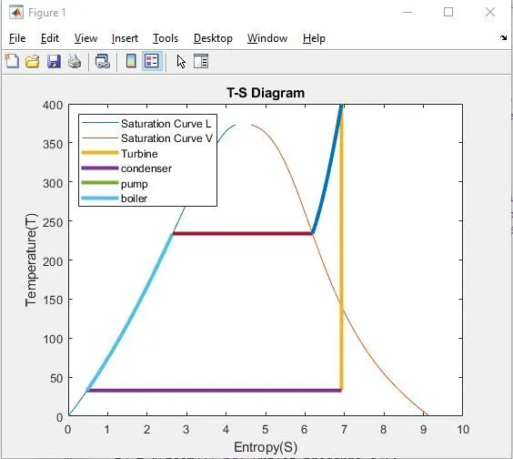
11. Now T-S diagram needs to be plotted with 4-5 and 6-1 process having curve lines and the required function for the same is given below;
hold on # To hold the entire plots in one figure
plot([s1 s2],[Inlet_temp t2],'linewidth',3) # To plot the 1->2 process,which will be a straight line
plot([s2 s3],[t2 t3],'linewidth',3)
plot([s3 s4],[t3 t4],'linewidth',3) # Similarly 2->3 and 3->4 lines are also plotted
tc1 = linspace(t4,t5,1000); # Sincethe 4->5 process is a curve, we try to plot the entropy for each values of temperature ie 1000 intervels
pc1 = linspace(p4,p5,1000);
for i=1:length(tc1) # Then for loop is created inorder to run for 1000 times
sc1(i) = XSteam('s_pT',pc1(i),tc1(i)); # entropy is calculated with pressure and temperature as the input.
end
plot(sc1,tc1,'linewidth',3)
plot([s5 s6],[t5 t6],'linewidth',3) # Plot for 5->6 process
tc2 = linspace(t6,Inlet_temp,1000); # simialr for 4->5, 6->1 also has to be plotted with a curve
pc2 = linspace(p6,Inlet_pressure,1000);
for i=1:length(tc2)
sc2(i) = XSteam('s_pT',pc2(i),tc2(i));
end
plot(sc2,tc2,'linewidth',3)
xlabel('Entropy(S)')
ylabel('Temperature(T)') # X axis and Y axis names are given
legend('Saturation Curve L','Saturation Curve V','Turbine','condenser','pump','boiler','location','northwest') # Legends are given to understand each process clearly
title('T-S Diagram') # Title of the plot is given
12. Same as that of what we have done above,saturation curve and H-S diagram has to be plotted w.r.t Enthalpy as the function in place of entropy in the former function.
Only difference is that curve lines has to be devoloped on 2->3,4->5,5->6 and 6->1 process.
GRAH PLOTS:
T-S DIAGRAM:
H-S DIAGRAM:
COMMAND WINDOW OUTPUT:
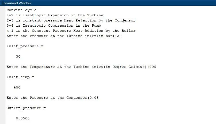
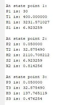
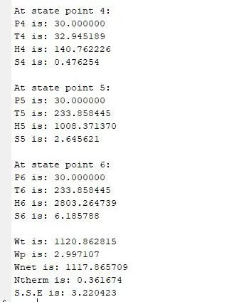
ERRORS FORMED:
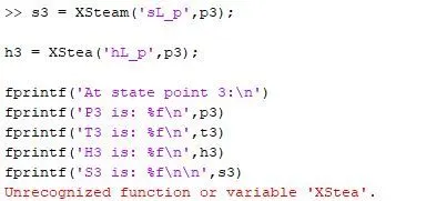

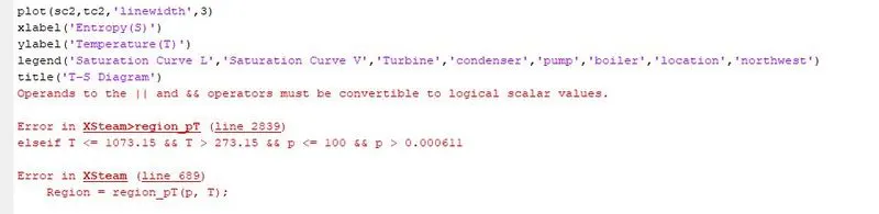
The normal syntax errors with error in case sensitive characters and paranthesis errors are encountered during the time of coding.
CONCLUSION:
- Learned about new syntax and function like XSteam which can be effectivily used for many other coding purposes.
- Simulated rankine cycle with TS and HS plots and understtod all the processes in between that.