Project 2 - Rankine cycle Simulator

RANKINE CYCLE: The Rankine cycle is a model used to predict the performance of steam turbine systems. It was also used to study the performance of reciprocating steam engines. The Rankine cycle is an idealized thermodynamic cycle of a heat engine that converts heat into mechanical work while undergoing phase change.

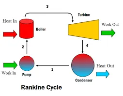
PROCESS OF RANKINE CYCLE:

• 1-2-3 Isobaric Heat Transfer. High pressure liquid enters the boiler from the feed pump (1) and is heated to the saturation temperature (2). ...
• 3-4 Isentropic Expansion. ...
• 4-5 Isobaric Heat Rejection. ...
• 5-1 Isentropic Compression.

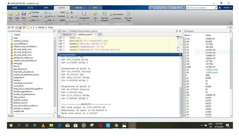
• %program to calculate the net work output and work back ratio
  %..for an rankine cycle and simulate t-s and h-s plot.
  
  %take user inputs 
  t3=input('enter turbine inlet temperature in (celcius)n');
  p3=input('enter turbine inlet pressure in(bar)n');
  p4=input('enter turbine outlet pressure in(bar)n');
  
  %processes are
  %1-2 isentropic compression
  %2-3 constant pressure heat addition
  %3-4 isentropic expansion
  %4-1 constant pressure heat rejection
  
  %calculate enthalpy at pt.3
  h3=xsteam('h_pt',p3,t3);
  
  %calculate enthalpy at pt.1
  hf1=xsteam('hl_p',p4);
  
  %calculate entropy at pt.3
  s3=xsteam('s_pt',p3,t3);
  
  %as line 3-4 is isentropic 
  s4=s3;
  
  %calculate entropy at pt.1
  sf1=xsteam('sl_p',p4);
  
  %calculating entropy diff at 0.005 bar 
  sfg4=xsteam('sv_p',p4)-xsteam('sl_p',p4);
  
  %calculating quality of steam at pt.4
  x=(s4-sf1)/sfg4;
  
  %enthalpy diff at 0.005 bar
  hfg4=xsteam('hv_p',p4)-xsteam('hl_p',p4);
  
  %enthalpy at pt.4
  h4=hf1+(x*hfg4);
  
  %work out at turbine 
  wt=h3-h4;
  
  %specific volume at pt.1
  vf=xsteam('vl_p',p4)
  
  %work consumed by pump
  wp=vf*(p3-p4);
  
  %total work output 
  wnet=wt-wp;
  
  %enthalpy at saturation liquid of pt.2
  hf2=wp+hf1;
  
  %heat input to boiler 
  qh=h3-hf2;
  
  %efficiency of cycle
  eff=(wnet/qh)*100;
  
  %back work ratio 
  bac=wp/wt;
  
  %properties at pt.1
  t1=xsteam('t_ps',p3,s1);
  p2=p3;
  h2=xsteam('h_ps',p3,s1);
  s2=s1;
  
  %properties at pt.3
  t3;
  p3;
  h3;
  s3;
  
  %properties at pt.4
  t4=xsteam('t_ph',p4,h4);
  p4;
  h4;
  s4;
  
  %properties of intermediate pts.b/w process 2-3
  t5=xsteam('tsat_p',p3);
  p5=p3;
  h5=xsteam('hl_p',p3);
  s5=xsteam('sl_p',p3);
  t6=xsteam('tsat_p',p3);
  p6=p3;
  h6=xsteam('hv p',p3);
  s6=xsteam('sv_p',p3);
  
  %%outputs
  
  fprintf('process 1-2 isentropic compression');
  fprintf('process 2-3 constant pressure heat addition');
  fprintf('process 3-4 isentropic expansion');
  fprintf('process 4-1 constant pressure heat rejection');
  
  fprintf('properties at point 1:n');
  fprintf('t1=%f (celciusn',t1);
  fprintf('p1=%f barn',p2);
  fprintf('h1=%f kj/kgn',h1);
  fprintf('s1=%f kj/kg cnn',s1);
  
  fprintf('properties at point 2:n');
  fprintf('t2=%f (celciusn',t1);
  fprintf('p2=%f barn',p2);
  fprintf('h2=%f kj/kgn',h2);
  fprintf('s2=%f kj/kg cnn',s2);
  
  
  fprintf('properties at point 3:n');
  fprintf('t3=%f (celciusn',t3);
  fprintf('p3=%f barn',p3);
  fprintf('h3=%f kj/kgn',h3);
  fprintf('s3=%f kj/kg cnn',s3); 
  
  fprintf('properties at point 4:n');
  fprintf('t4=%f (celciusn',t4);
  fprintf('p4=%f barn',p4);
  fprintf('h4=%f kj/kgn',h4);
  fprintf('s4=%f kj/kg cnn',s4);
  
  fprintf('results n ');
  fprintf('net work output is %f kjn',wnet);
  fprintf('efficiency of cycle is %f %n',eff);
  fprintf('back work ratio is %f ',bac);
  
  %%plotting t-s and h-s plot 
  %plotting saturation line 
  t=(1:2000);
  for i=1:1:2000
      sl(1,i)=xsteam('sl_t',i);
      sv(1,i)=xsteam('sv_t',i);
      hl(1,i)=xsteam('hl_t',i);
      hv(1,i)=xsteam('hv_t',i);
  end
  figure(1)
  plot(sl,t,'b','linewidth',1);
  hold on;
  plot(sv,t,'b','linewidth',1);
  xlabel('entropy (kj/kg c)');
  ylabel('temperature (c)');
  title('temperature vs entropy plot');
  
  figure(2)
  plot(sl,t,'b','linewidth',1);
  hold on;
  plot(sv,t,'b','linewidth',1);
  xlabel('entropy (kj/kg c)');
  ylabel('enthalpy(kj/kg)');
  title('enthalpy vs entropy plot');
  
  %ploting the rankine cycle 
  figure(1)
  plot([s1,s2,s5,s6,s3,s4,s1],[t1,t2,t5,t6,t3,t4,t1],'k','linewidth',1);
  figure(2)
  plot([s1,s2,s5,s6,s3,s4,s1],[h1,h2,h5,h6,h3,h4,h1],'k','linewidth',1);

• outputs:
• 1.we get the net work output as 1120.83 kj
• 2.effficiency of cycle as 36.22%
• 3.back work ratio is 0.000027
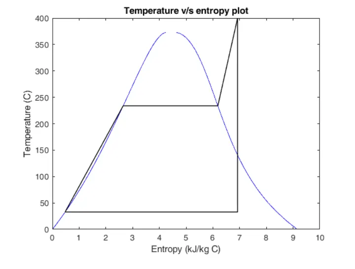
• 4.temperature vs entropy plot
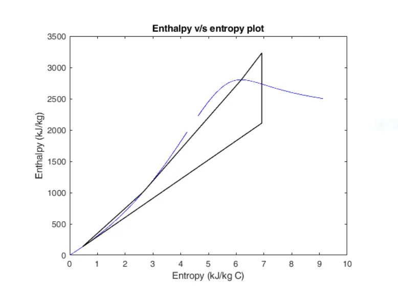
• 5.enthalpy vs entropy plot
• output images:
•