Project 2 - Rankine cycle Simulator

Main Code -

clear all
close all
clc
% USER INPUTS
disp('                     RANKINE CYCLE SIMULATOR');
P1 = input('\nEnter the pressure at the turbine inlet(in bar):');
T1 = input('\nEnter the temperature at the turbine inlet(in Degree Celsius):');
P2 = input('\nEnter the pressure at the condenser(in bar):');

% Initial State Calculations i.e. input to turbine  

H1 = XSteam('h_pT',P1,T1);
S1 = XSteam('s_pT',P1,T1);
fprintf('\n')
disp('                           RESULTS');
disp('At State Point 1')
fprintf('\nP1 is :%f bar',P1)
fprintf('\nT1 is :%f degree celsius',T1)
fprintf('\nH1 is :%f KJ/Kg',H1)
fprintf('\nS1 is :%f KJ/KgK\n\n',S1)

% Second State Calculations i.e. Turbine output 

S2 = S1;
H2 = XSteam('h_ps',P2,S2);
T2 = XSteam('t_ps',P2,S2);
Sf = XSteam('sL_p',P2); % liquid entropy at P2
Sg = XSteam('sV_p',P2); % vapour entropy at P2
Sfg = Sg - Sf;
X2 = (S2-Sf)/Sfg; % Quality of mixture
disp('At State Point 2')
fprintf('\nP2 is :%f bar',P2)
fprintf('\nT2 is :%f degree celsius',T2)
fprintf('\nH2 is :%f KJ/Kg',H2)
fprintf('\nS2 is :%f KJ/KgK',S2)
fprintf('\nX2 is :%f \n\n',X2)

% Third State Calculations i.e. Condenser output 

P3 = P2;
T3 = T2;
H3 = XSteam('hL_p',P3);
S3 = XSteam('sL_p',P3); 
disp('At State Point 3')
fprintf('\nP3 is :%f bar',P3)
fprintf('\nT3 is :%f degree celsius',T3)
fprintf('\nH3 is :%f KJ/Kg',H3)
fprintf('\nS3 is :%f KJ/KgK\n\n',S3)
        
% Fourth State Calculations i.e. Pump output 

S4 = S3;
P4 = P1;
T4 = XSteam('T_ps',P4,S4);
H4 = XSteam('h_ps',P4,S4); 
disp('At State Point 4')
fprintf('\nP4 is :%f bar',P4)
fprintf('\nT4 is :%f degree celsius',T4)
fprintf('\nH4 is :%f KJ/Kg',H4)
fprintf('\nS4 is :%f KJ/KgK',S4) 

% work, efficiency, specific steam consumption 
Wt = H1 - H2; % Turbine Work
Wp = H4 - H3; % Pump Work
Wnet = Wt - Wp; % Net Work Done
Heat_input = H1 - H4; 
Heat_output = H2 - H3;
Ntherm = (1-(Heat_output/Heat_input))*100; % Thermal Efficiency
SSC = (1/Wnet)*3600; %specific steam consumption
fprintf('\n\nWt is :%f KJ/Kg',Wt)
fprintf('\nWp is :%f KJ/Kg',Wp)
fprintf('\nWnet is :%f KJ/Kg',Wnet)
fprintf('\nNtherm is :%f Percent',Ntherm)
fprintf('\nS.S.C. is :%f Kg/KWh',SSC)

% T-s Graph Plot
plot([S1,S2],[T1,T2],[S2,S3],[T2,T3],[S3,S4],[T3,T4],'color','b')
figure(1)
hold on
plot_points = linspace(S4,S1,5000);
for i = 1:length(plot_points)
    T_Plot(i) = XSteam('T_ps',P4,plot_points(i));
    S_Plot(i) = plot_points(i);
end
ax1 = plot(S_Plot,T_Plot,'color','b','DisplayName','Rankine Cycle Plot');

% Saturation Liquid Line
for j = 0:2000
if isnan(XSteam('sL_T',j))
    continue
else
    break
end
end

first_temp_point_liquid = j;

for j = 2000:-1:0
if isnan(XSteam('sL_T',j))
    continue
else
    break
end
end

last_temp_point_liquid = j;

k = 1;
Temperature_range_liquid = first_temp_point_liquid:1:last_temp_point_liquid;
for m = Temperature_range_liquid
saturation_entropy_liquid(k) = XSteam('sL_T',m);
k = k+1;
end

% Saturation Vapour Line
for j = 0:2000
if isnan(XSteam('sV_T',j))
    continue
else
    break
end
end

first_temp_point_vapour = j;

for j = 2000:-1:0
if isnan(XSteam('sV_T',j))
    continue
else
    break
end
end

last_temp_point_vapour = j;

k = 1;
Temperature_range_vapour = first_temp_point_vapour:1:last_temp_point_vapour;
for m = Temperature_range_vapour
saturation_entropy_vapour(k) = XSteam('sV_T',m);
k = k+1;
end

ax2 = plot(saturation_entropy_liquid,Temperature_range_liquid,saturation_entropy_vapour,Temperature_range_vapour,'color','r');
title('T-S Diagram')
ylabel('Temperature (°C)')
xlabel('Entropy (KJ/KgK)')
legend([ax1(1),ax2(1)],'Rankine Cycle Plot','Saturation Line','Location','NorthEastOutside')
labels = {'1'};
text(S1,T1,labels,'VerticalAlignment','bottom','HorizontalAlignment','left')
labels = {'2'};
text(S2,T2,labels,'VerticalAlignment','top','HorizontalAlignment','left')
labels = {'3'};
text(S3,T3,labels,'VerticalAlignment','top','HorizontalAlignment','left')
labels = {'4'};
text(S4,T4,labels,'VerticalAlignment','bottom','HorizontalAlignment','right')
% h-s Graph Plot
figure(2)
hold on
plot_points = linspace(S4,S1,5000);

for i = 1:length(plot_points)
    T_Plot = XSteam('h_ps',P4,plot_points(i));
    plot(plot_points(i),T_Plot,'color','b')
end

plot([S1,S2],[H1,H2],[S3,S4],[H3,H4])

plot_points = linspace(S2,S3,5000);

for i = 1:length(plot_points)
    T_Plot = XSteam('h_ps',P2,plot_points(i));
    ax3 = plot(plot_points(i),T_Plot,'color','b');
end

% Saturation Liquid Line
k = 1;
Temperature_range = first_temp_point_liquid:1:last_temp_point_liquid;
for m = Temperature_range
saturation_enthalpy_liquid(k) = XSteam('hL_T',m);
k = k+1;
end
plot(saturation_entropy_liquid,saturation_enthalpy_liquid,'color','r')

% Saturation Vapour Line
k = 1;
Temperature_range = first_temp_point_vapour:1:last_temp_point_vapour;
for m = Temperature_range
saturation_enthalpy_vapour(k) = XSteam('hV_T',m);
k = k+1;
end
ax4 = plot(saturation_entropy_vapour,saturation_enthalpy_vapour,'color','r');
title('H-S Diagram')
ylabel('Enthalpy (KJ/Kg)')
xlabel('Entropy (KJ/KgK)')
legend([ax3,ax4],'Rankine Cycle Plot','Saturation Line','Location','NorthEastOutside')
labels = {'1'};
text(S1,H1,labels,'VerticalAlignment','bottom','HorizontalAlignment','left')
labels = {'2'};
text(S2,H2,labels,'VerticalAlignment','top','HorizontalAlignment','left')
labels = {'3'};
text(S3,H3,labels,'VerticalAlignment','top','HorizontalAlignment','left')
labels = {'4'};
text(S4,H4,labels,'VerticalAlignment','bottom','HorizontalAlignment','right')

Output -

• Command Window -

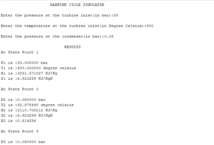
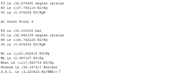
• Graphs Output (Colour has faded on converting it to image for one of plot line)

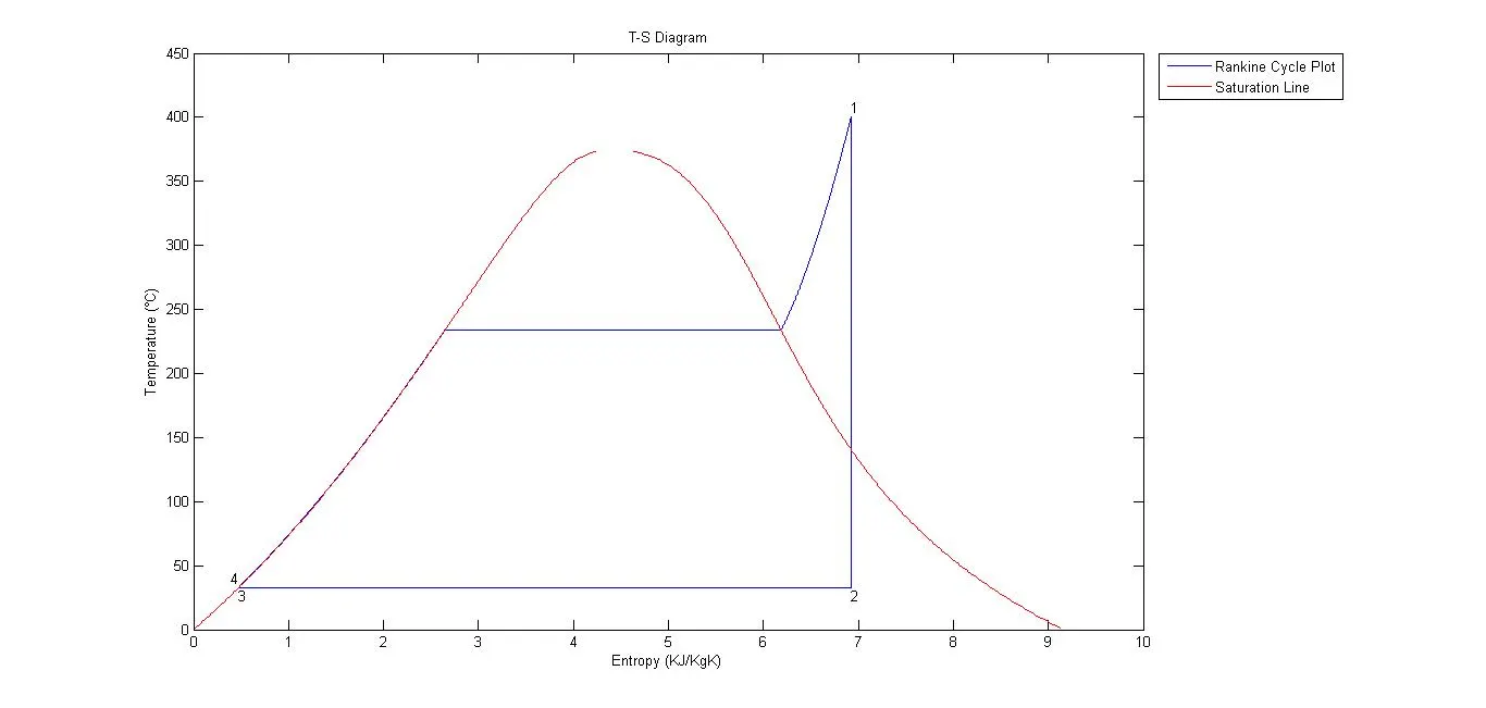
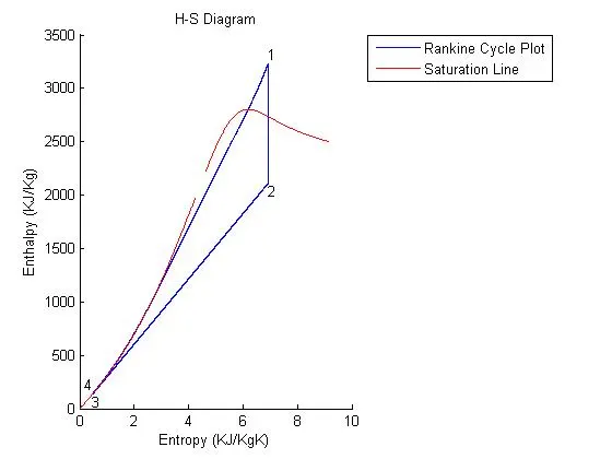
Rankine Cycle Working : Due to limitations in carnot cycle such as low quality steam (can damage turbine blades over time) and isothermal heat transfer at various pressures as well as designing a compressor which can handle two phases, rankine cycle is used. Although, efficiency would be lower than carnot cycle, but it will be practical. In this cycle working fluid is compressed by pump (isentropic compression). Since, this is liquid state it is almost incompressible. Since, change in temperature is zero in case of isentropic process for incompressible substance, there will be a minor temperature change. After that this fluid is injected in boiler for constant pressure heat addition. At the end of process we have superheated vapour as working substance, which is further injected into turbine. Since, steam does work on turbine and has no heat addition, this is isentropic process. Thus, isentropically working substance cools by delivering work. From there it is then sent to condensor where heat rejection at constant pressure takes place which brings the working substance to initial state.

Code Explanation -

Main Code - First, clear all, close all and clc is used to clear all variables, command windows and close all windows. Then, required user inputs are taken throught input command. Then, through xsteam library state functions of first state are calculated and printed. Similarly, through xsteam library state functions of second, third and fourth state are calculated and printed. In second state steam quality is also calculated. Then, the results of turbine work, pump work, net wotk, thermal efficiency and specific steam consumption are calculated through suitable thermodynamic formulas and printed. Then, temperature-entropy graph is plotted. For plotting the straight lines of three states plot command is used. For plotting the variable line of constant pressure heat addition for loop is used wherein temperature value at each point is calculated through Xsteam wherein input points are taken from linspace command between end points. Then, saturation line is plotted. For this, valid temperature range is first calculated. Xsteam has temperature range of 0 to 2000 degrees celsius. Using for loop, it is calculated for which first value of temperature NaN is not received. That value is intial temperature value. Again for loop is applied in decreasing fashion to find first valid value which is final temperature value. Then, entropy values corresponding to these values are calculated and plotted. This is done seperate for vapour and liquid line. Then, legend, axis and labels are defined.

Now, enthalpy-entropy graph will be plotted. For plotting the straight lines of two states plot command is used. For plotting the variable line of constant pressure heat addition for loop is used wherein enthalpy value at each point is calculated through Xsteam wherein input points are taken from linspace command between end points. For plotting the variable line of constant pressure heat rejection for loop is used wherein enthalpy value at each point is calculated through Xsteam wherein input points are taken from linspace command between end points. Then, saturation line is plotted. For this, valid entropy range is already calculated. Using these values, enthalpy values corresponding to these values are calculated and plotted through Xsteam library. This is done seperate for vapour and liquid line. Then, legend, axis and labels are defined.

Error Encountered -

"Error using horzcat
Dimensions of matrices being concatenated are not consistent.

Error in rankine_cycle (line 148)
legend([ax1(1),ax2],'Rankine Cycle Plot','Saturation Line','Location','NorthEastOutside')"

Screenshot -

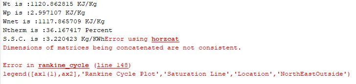
Error Troubleshooting - Error ocurred because second handle defined is 2x1 matrix and first handle defined is 1x1 matrix. In, order to concatenate we can use ax2(1) along with ax1(1) so that both the handles are for same dimension for legend operation.

References -

1. Thermodynamics : An Engineering Approach, Yunus A. Cengel, Michael A. Boles, McGraw Hill Education.