Project 2 - Rankine cycle Simulator
Aim:
To create ideal Rankine cycle simulator.
Objectives:
- Calculating state points of the Rankine cycle based on user input.
- Plotting corresponding T-s and h-s diagram.
Theory:
Rankine cycle is a model widely used by power plants, where a fuel is used to produce heat within the boiler so as to convert water into steam which then expands through a turbine producing useful work.
Assumptions:
- Boiler and condenser are constant pressure devices.
- Liquid at the condenser outlet is saturated.
- Steady operating conditions.
- Compression and expansion process is isentropic.
- Internal irreversibility is absent.
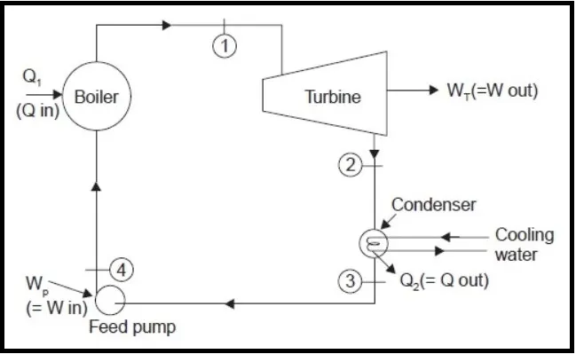
As, we can see from the fig., The steam at state1 enters the turbine and undergoes the isentropic expansion process. This decreases the temperature and pressure of the vapor thereby generating power. Here we have to make sure that the steam entering the turbine is superheated so that maximum output power can be generated and the turbine blades will not be harmed because of moisture. After leaving the turbine it enters into condenser where it rejects the heat to circulating cooling water, this is constant pressure process. After leaving condenser, saturated liquid enters the pump which compresses the liquid to boiler pressure & this is an isentropic process as well. In boiler, the heat is added at constant pressure till it becomes super saturated. The work done by the pump is considerably lower than the work obtained from the turbine.
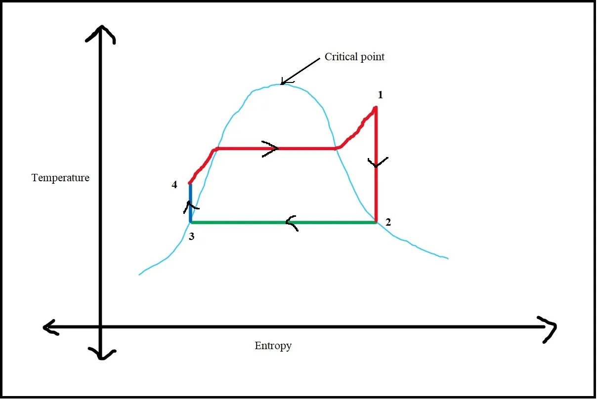
As given in the diagram, there are basically four processes as:
- Process1-2: Isentropic expansion in turbine.
- Process2-3: Constant pressure heat rejection in condenser.
- Process3-4: Isentropic compression in pump.
- Process4-1: Constant pressure heat addition in boiler.
According to specific enthalpy relation,
`dh = tds + nudp;`
for process1-2 in the turbine, as it is isentropic the change in entropy will be zero.
So, `dh =h1-h2 = nudp =` work obtained from turbine (Wt)
Where, `nu =` specific volume `(m^3/(kg))`.
`dp =` change in pressure.
Similarly, for process2-3 in the condenser as the process is at constant pressure so,
Heat rejected `= dq = dh = h2-h3`
Work done by pump `(Wp)= h4-h3`
Heat added in boiler `= h1-h4`
Net-Work output = Wnet = `Wt-Wp`
Back work ratio = `(Wp)/(Wt)`
Efficiency = `eta =`Wnet/Heat supplied
Body of content:
Now coming to the program, we are required to take the user inputs so we have used input command for the given data i.e. for t1, p1 and p2. This will ask the user to put the data so that the required parameters will be calculated accordingly.
Our next aim is to calculate the state variables at four points as shown in the fig. As point1 which is the entry to turbine can be saturated or superheated so we need to specify both temperature and pressure to get enthalpy(h) and entropy(s) values (from XSteam file). The command that we used to get sp. Enthalpy value is XSteam('h_pT',p1,t1); where letters just after the underscore sign represents the inputs that we are going to take to find respective values. At point2 which is entry to condenser, as the process is isentropic so entropy will be same. Temperature at state2 will be nothing but temperature at that saturation pressure which is already known from given data, but to calculate enthalpy value we will need both pressure value and dryness fraction. To calculate that we used the same command syntax as that for point1. Process2-3 is at constant pressure so p3 = p2 and then we can get h3, s3, t3 with p3 as input. Process3-4 is isentropic compression in pump so again s4 = s3 with p4 = p1 (because process4-1 is at constant pressure), then using that we can find out h4, t4 using command syntax given.
%% Ideal Rankine cycle simulator

%Process1-2= expansion in steam turbine
%Process2-3= heat rejection in condenser
%Process3-4= work done by pump
%Process4-1= heat addition in boiler

%h--> specific enthalpy (kJ/kg)
%s--> specific entropy (kJ/kg-K)
%t--> temperature (degree C)

clear all
close all
clc

%Input parameters
t1 = input('Eenter Turbine inlet temperature (in degree C):');
p1 = input('Enter Turbine inlet pressure (in bars):');
p2 = input('Enter Condenser inlet temperature (in bars):');

%% Calculating state variables

%at point1
h1 = XSteam('h_pT',p1,t1);   %finding sp. enthalpy from XSteam corresponding to p1 & t1
s1 = XSteam('s_pT',p1,t1);


%at point2
s2 = s1;
x2 = XSteam('x_ps',p2,s2);  %dryness fraction at point2.
t2 = XSteam('Tsat_p',p2);
h2 = XSteam('h_px',p2,x2);


%at point3
p3 = p2;
h3 = XSteam('hL_p',p3);
s3 = XSteam('sL_p',p3);
t3 = XSteam('Tsat_p',p3);


%at point4
s4 = s3;
p4 = p1;
t4 = XSteam('T_ps',p4,s4);
h4 = XSteam('h_pT',p4,t4);
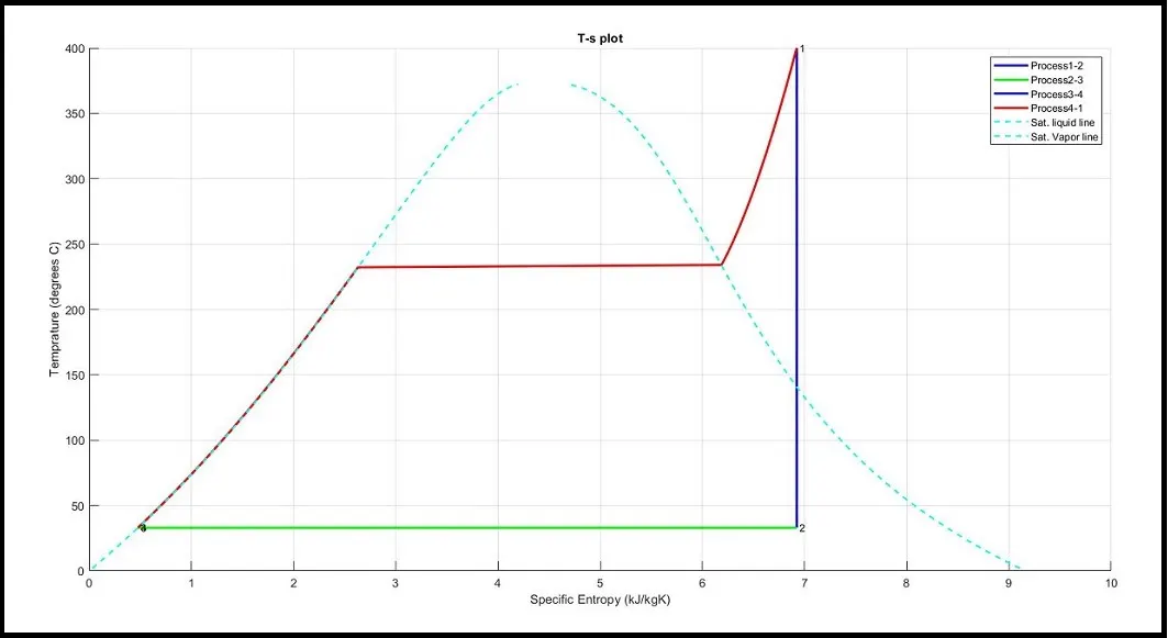
As we have already calculated state variables our next step plotting. Figure (1) is T vs s diagram. We already know the temperature and entropy at the state points and with the fact that process1-2, process2-3 and process3-4 are just the straight lines we can directly join those respective points. For that we have directly used plot command with respective state points values of entropy and temperature. Process4-1 is not at all just a straight line so we have to calculate entropy values for respective temperatures. To do this we split the temperature range from t1 to t4 into 200 parts with the help of linspace command. Then we have to use for loop to take each value of temperature and again in for loop we used the XSteam syntax to find out respective values from XSteam file. We stored the specific enthalpy values for process2-3, 4-1 in array H_23 and H_41 respectively, we have also stored sp. Entropy values (for both the process) in S array. Now to plot process4-1, we took S and T_41 as input. After that we have used text command to name the respective state points.
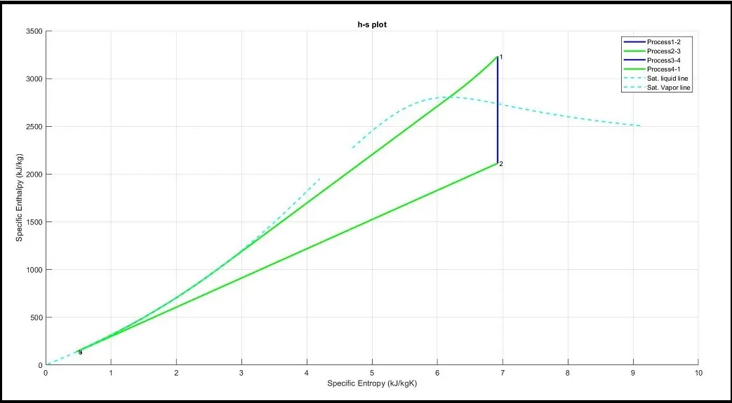
Similarly, for h vs s diagram we have directly used state point values for process1-2 and 3-4 while we need to use array values as calculated earlier for process2-3 & 4-1.
Now to plot saturated vapor and saturated liquid curve, we need the reference of critical point of water which is equal to 374.15 degree Celsius. Again, we have divided 0 to 347.15 temperature range into 200 parts using linspace command and saved those into T_sat array. Again, using for loop we have found out sat. liquid and sat. vapor entropy values at all the points in that temperature range and stored those values into Sl and Sv array respectively. Then taking those arrays as reference we have plotted the vapor dome in T-s plot. To plot sat. liquid and sat. vapor curve in h-s plot we have followed the similar procedure by just replacing Sl and Sv by Hl and Hv respectively.
%% Plotting for T vs s diagram
figure(1)
hold on
plot([s1 s2],[t1 t2],'color','b','linewidth',2);
plot([s2 s3],[t2 t3],'color','g','linewidth',2);
plot([s3 s4],[t3 t4],'color','b','linewidth',2);
T_41 = linspace(t4,t1,200);     %temp. array for process4-1
for i = 1:length(T_41)
    S(i) = XSteam('s_pT',p1,T_41(i));  %specific entropy array for process4-1(& 2-3)
    H_23(i) = XSteam('h_ps',p1,S(i));
    H_41(i) = XSteam('h_ps',p2,S(i));
end
plot(S,T_41,'color','r','linewidth',2);    %plotting process4-1
xlabel('Specific Entropy (kJ/kgK)')
ylabel('Temprature (degrees C)')
title('T-s plot')
text(s1,t1,' 1','FontSize',9)  %naming the respecting points
text(s2,t2,' 2','FontSize',9)
text(s3,t3,' 3','FontSize',9)
text(s4,t4,' 4','FontSize',9)
grid on


%% Plotting for h vs s diagram
figure(2)
hold on
plot([s1 s2],[h1 h2],'color','b','linewidth',2);
plot(S,H_23,'color','g','linewidth',2);     %plotting process2-3
plot([s3 s4],[h3 h4],'color','b','linewidth',2);
plot(S,H_41,'color','g','linewidth',2);
xlabel('Specific Entropy (kJ/kgK)')
ylabel('Specific Enthalpy (kJ/kg)')
title('h-s plot')
text(s1,h1,' 1','FontSize',9)
text(s2,h2,' 2','FontSize',9)
text(s3,h3,' 3','FontSize',9)
text(s4,h4,' 4','FontSize',9)
grid on


%% Ploting sat. liquid and sat. vapor curve in T vs s diagram
T_sat = linspace(0,374.15,200);
figure(1)
hold on
for i = 1:length(T_sat)
    Sl(i) = XSteam('sL_t',T_sat(i));    %sp. entropy array for sat. liq. region
    Sv(i) = XSteam('sV_t',T_sat(i));
end

plot(Sl, T_sat, 'color','c', 'linestyle', '--', 'linewidth', 1.5)
plot(Sv, T_sat, 'color','c', 'linestyle', '--', 'linewidth', 1.5)
legend('Process1-2', 'Process2-3', 'Process3-4', 'Process4-1', 'Sat. liquid line','Sat. Vapor line');

%% Ploting sat. liquid and sat. vapor curve in h vs s diagram
figure(2)
hold on
for i = 1:length(T_sat)
    Hl(i) = XSteam('hL_t',T_sat(i));
    Hv(i) = XSteam('hV_t',T_sat(i));    %sp. enthalpy array for sat. vapor region
end
plot(Sl, Hl, 'color','c', 'linestyle', '--', 'linewidth', 1.5)
plot(Sv, Hv, 'color','c', 'linestyle', '--', 'linewidth', 1.5)
legend('Process1-2', 'Process2-3', 'Process3-4', 'Process4-1', 'Sat. liquid line','Sat. Vapor line');
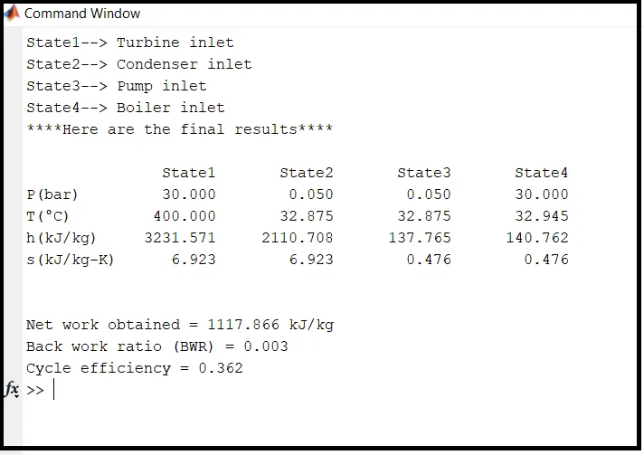
Now, we have calculated the required performance parameters using the formulas given. Coming to printing the final results, first of all we have clearly mentioned what does state points represents. To print the result in table form we have to leave some blank space before each column and as you can see to do that, we have associated a number just before respective datatype (here s and f). and so, printed the corresponding values. We have also printed performance parameters calculated earlier i.e. Net-Work, back work ratio and efficiency using fprintf command.
%% Calculating Performance parameters
W_turbine = h1 - h2;        %work obtained from turbine
W_pump = h4 - h3;
Q_rejected = h2 - h3;       %heat rejected by condenser
Q_supplied = h1 - h4;
Wnet = W_turbine - W_pump;
BWR = W_pump/W_turbine;     % Back work ratio
eta = Wnet/Q_supplied;      % Rankine cycle efficiency

clc
%% Final results
fprintf('State1--> Turbine inlet n');
fprintf('State2--> Condenser inlet n');
fprintf('State3--> Pump inlet n');
fprintf('State4--> Boiler inlet n');

fprintf('****Here are the final results**** nn');

fprintf('%21s %12s %12s %12sn', 'State1', 'State2', 'State3', 'State4');
fprintf('%2s %14.3f %12.3f %12.3f %12.3f n','P(bar)',p1,p2,p3,p4);
fprintf('%2s %15.3f %12.3f %12.3f %12.3f n','T(°C)',t1,t2,t3,t4);
fprintf('%2s %12.3f %12.3f %12.3f %12.3f n','h(kJ/kg)',h1,h2,h3,h4);
fprintf('%2s %10.3f %12.3f %12.3f %12.3f nnn','s(kJ/kg-K)',s1,s2,s3,s4);

fprintf('Net work obtained = %.3f kJ/kg n',Wnet);
fprintf('Back work ratio (BWR) = %.3f n',BWR);
fprintf('Cycle efficiency = %.3f  n',eta);
Results:
Temperature vs Specific entropy plot:
Specific enthalpy vs Specific entropy plot:
Output in command window:
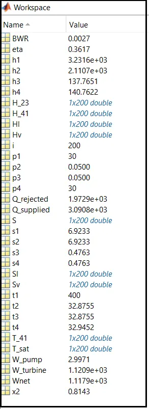
Output in workspace:
Conclusion:
Thus, the state point properties are calculated using XSteam library (MATLAB file) and using that T-s and h-s diagrams are plotted. Performance parameters like Net-Work, Back work ratio (BWR) and efficiency of cycle is also found out.
Errors:
I missed a parenthesis in a line, which was rectified.
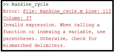
I was unable to get the value of h2 with p2, s2 as inputs but later I included steam fraction x2 along with p2 as inputs, and the problem got rectified.
Reference: