Many embedded systems need to track their own location or position and heading, and designers often turn to GNSS (Global Navigation Satellite Systems) as a first resort (see, “Design Location Tracking Systems Quickly Using GNSS Modules”). However, GPS cannot always be used exclusively for position and heading information for several reasons, starting with power consumption.
GPS systems draw significant amounts of power. Many embedded systems, especially battery powered, cannot afford the power budget needed to maintain a GPS position 100 percent of the time. In addition, GPSs suffer from signal blockages, slow update rates, and an accuracy of 1 meter (m) that might not be sufficient for some applications.
These problems can be overcome by using inertial measurement units (IMUs) to complement GNSS position data.
A previous IMU article discussed the use of relatively inexpensive IMUs based on MEMs technology for determining position and heading, see “Use IMUs for Precise Location Data When GPS Won’t Suffice”. However, IMU sensor data alone cannot provide absolute position. While GNSS receivers simply provide location data, a significant amount of software is required to convert an IMU’s relative motion data into an absolute position and heading using sensor filtering, fusion, and double integration.
This article discusses the embedded use of IMUs, sources of error in the data from various IMU sensors, and the software needed to calculate precise location and heading information from IMU sensors. In addition, this article discusses the STMicroelectronics MotionFX library and how to use this software to transform IMU sensor data into position and heading within an embedded system.
How IMUs complement GNSS receivers
The problems with GNSS are fourfold:
GNSS signals are very directional and are easily blocked by buildings. Therefore, GNSS operation indoors or deep within urban concrete canyons can be problematic.
GNSS receivers have warm and cold startup times measured in the tens of seconds or more. If the GNSS receiver is not operated continuously, to save energy for example, then each new position reading can take multiple seconds.
GNSS’ position update rate is limited to once per second. This update rate is not sufficiently frequent for embedded applications involving quick movement. There’s a long list of such applications ranging from virtual reality to materials handling and robotics.
GNSS accuracy is measured in meters. That resolution is far too coarse for use in many embedded applications.
IMUs provide the finer positioning resolution and faster update rates that are required by many embedded applications. Also, IMUs provide relative position data from a known starting point as opposed to the absolute positioning information from a GNSS receiver, so the two types of position sensors complement each other. These IMU characteristics make them quite useful for augmenting the positioning information obtained directly from GNSS receivers, see “Design Location Tracking Systems Quickly Using GNSS Modules”.
IMUs have existed in the aerospace industry for many decades. However, these precision aerospace IMUs are based on expensive gyroscopes and other large sensors, and are difficult to apply to more cost-sensitive systems.
Modern electronic IMUs are highly integrated and can contain a mix of sensor types—accelerometers, gyroscopes, and magnetometers—which are based on microelectromechanical systems (MEMS) technology so they’re small, light, and relatively rugged. These new generations of IMUs are available as board mountable components and are proving to be ideal for embedded applications.
IMUs come with varying capabilities in terms of degrees of freedom (DOF), and unlike GNSS receivers, IMUs do not depend upon radio signals for position data. They also consume very little power and they’re available from a variety of sources with a wide range of resolution and accuracy specifications.
With these characteristics, IMUs can be used to augment positioning information from GNSS receiver modules (see, “Design Location Tracking Systems Quickly Using GNSS Modules”), but not without a significant amount of software to filter the IMU sensor data, to fuse sensor data from the several types of sensors inside the IMU, and to calculate a position from that fused sensor data using double integration.
Sources of IMU error
Combining sensors to improve accuracy has long been a common practice in the aerospace industry, where accelerometers and gyroscopes are extensively used in inertial navigation systems. In these systems, gyroscopes sense orientation through angular velocity changes, but they tend to drift over time because they only sense changes and have no fixed frame of reference. Adding accelerometer data to the gyroscope data allows the gyroscope bias to be minimized, resulting in a more accurate location estimate. Accelerometers sense changes in direction with respect to gravity, and that data can be used to orient a gyroscope.
Accelerometers are more accurate for static (as opposed to dynamic) calculations. Gyroscopes are better at detecting orientation when the system is already in motion. Accelerometers react quickly, so accelerometer jitter and noise produce accumulated error when that data is used alone. In addition, accelerometers tend to distort accelerations due to external forces such as gravitational forces, which also accumulate in the system as noise.
Combining a gyroscope’s short-term accuracy with an accelerometer’s long-term accuracy results in more precise orientation readings by relying on each sensor’s strengths to cancel or at least reduce the other sensor’s weaknesses. The two sensor types complement each other.
Fused filtering needed to reduce error
IMU software uses filtering to minimize positioning error from IMU data. Several filtering methods for fusing sensor data are available, each with varying degrees of complexity. A complementary filter is a simple way to combine data from several sensors. Complementary filtering is a linear function that combines a high pass gyroscope filter and low pass accelerometer filter. High frequency noise in the accelerometer data is therefore filtered out in the short term and smoothed by the gyroscope data.
While the complementary filter is computationally simple, more involved techniques such as the Kalman filter are now preferred for IMU use to achieve better accuracy. The Kalman filter is a very popular recursive sensor fusion algorithm because it does not take a lot of processing power to create a more accurate positioning system. There are different types of Kalman filtering including the standard Kalman filter, the extended Kalman filter (EKF) and the unscented Kalman filter (UKF).
A Kalman filter predicts values using several mathematical equations based on the assumption that the data being filtered takes the form of a Gaussian distribution, to which the filter applies linear equations. However, motion in the real world is not as clean as the Kalman filter’s assumption. Real-world motion adheres to equations often involving sine and cosine functions which are nonlinear, so the EKF employs a Taylor series and single point approximations of the Gaussian distribution to linearize nonlinear functions. These approximations can be significant error sources.
The UKF addresses this error problem by using a deterministic sampling approach that generates a set of carefully chosen sample points to represent expected Gaussian distribution of the data rather than the single approximation used by the EKF. These sample points completely capture the true mean and covariance of the expected Gaussian values and result in more accurate filtering.
Magnetometer error sources
A typical IMU contains three different sensors: a gyroscope to measure angular rate/velocity, an accelerometer to measure linear acceleration, and a magnetometer to measure magnetic field strength. More specifically, the IMU’s magnetometers measure the earth’s magnetic field strength to determine a heading relative to the earth’s magnetic north. An IMU designed for navigation applications will usually contain three of each type of sensor, to cover the three orthogonal motion axes.
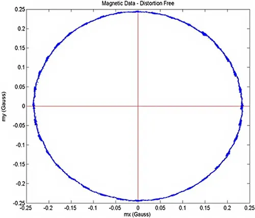
However, magnetometers are susceptible to hard iron and soft iron distortions. Distortions of the earth's magnetic field that result from external magnetic influences are generally classified as either a hard iron or soft iron effect. If no distorting effects are present, rotating a magnetometer through 360° and plotting the resulting data will result in data that forms a circle centered around (0, 0) (Figure 1).
Figure 1: Rotating a magnetometer through 360° and plotting the resulting data will result in data that forms a circle centered on location (0, 0), if there are no local field distortions caused by nearby iron. (Image source: sensorsmag.com)
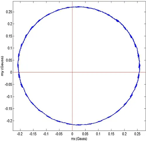
The presence of hard iron and/or soft iron effects may disturb the circle. Hard iron effects cause a simple offset from location (0, 0) (Figure 2).
Figure 2: A hard iron distortion effect offsets the magnetic data from location (0, 0). (Image source: sensorsmag.com)
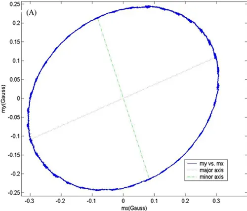
Soft iron effects deform the circle to produce an ellipse (Figure 3).
Figure 3: A soft iron distortion effect distorts the 360° magnetic data, changing it from a circle into an ellipse. (Image source: sensorsmag.com)
Note that both hard and soft iron effects can appear simultaneously.
The calculations that compensate for soft iron distortion are more compute intensive than those required to compensate for hard iron distortion, so it may be more efficient and cost effective simply to move soft iron materials away from the IMU’s magnetometers. However, in many cases this is not an option and compensation calculations will be required.
Integrate, then integrate again
Finally, because the accelerometers and gyroscopes only provide information about the acceleration forces (linear and rotary) on an object, that data must be integrated twice to produce location because acceleration is the rate of change of an object’s velocity, and velocity is the rate of change of an object’s position. In other words, IMU gyroscope and accelerometer data provide the double derivatives of an object’s absolute location.
Double integration alone requires a fair bit of processing, but for 3D positioning the acceleration effects of gravity must be nulled out as well. Gravity looks like a constant acceleration to an accelerometer, resulting in an offset in its data. Usually, the acceleration effects of gravity must be calibrated out of the system while the IMU and the object containing the IMU are at rest.
Note that there will be errors caused by this double integration due to sampling error. The slower the sample rate, the greater the error.
Design considerations for IMU software
Consider the following steps and recommendations when implementing these kinds of algorithms for real-world IMU software:
IMU sensor signals are not free of noise and will require digital filtering. Typically, some sort of Kalman filtering is used in IMU applications.
Even with filtering, additional error sources will be present such as mechanical noise coupled to the IMU, and the hard iron and soft iron distortion discussed above. This noise must be filtered out or otherwise removed from the data.
A calibration routine performed while the IMU is at rest will be required at the start of the application because to be as accurate as possible, the software will need to know what the sensor readings are when the object is not moving. The real acceleration value for an object in motion is the current sample from an acceleration sensor minus the calibration value.
After calibration, sensor values can be either positive or negative. Therefore, variables to hold these values must be signed.
A faster sampling frequency for the sensor data produces more accurate results, but more samples will require more memory, tighter timing requirements, and perhaps other hardware considerations.
The sampling period must always be precisely the same. Unequal sample periods will cause data errors.
Linear data approximation between samples (interpolation) produces more accurate results but also requires more processing time.
From the above discussion, it’s apparent that the calculations needed to determine heading, position, and motion from IMU data are not simple. For that reason, IMU vendors often offer software application packages to perform these calculations for their products. For example, STMicroelectronics has developed the MotionFX library which expands the capabilities of the company’s downloadable X-CUBE-MEMS1 software to encompass IMU functions.
Software in this library acquires data from the accelerometers, gyroscopes, and magnetometers and provides real-time motion sensor data fusion for STMicroelectronics' MEMS sensors, including IMUs. The MotionFX filtering and predictive software uses advanced algorithms to intelligently integrate outputs from multiple MEMS sensors, regardless of environmental conditions. This library is only designed for STMicroelectronics’ MEMS IMUs so the software’s functionality and performance are not assured when using IMUs from other vendors.
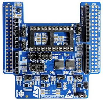
The MotionFX library runs on a variety of STMicroelectronics’ microcontrollers based on the Arm® Cortex®-M0+, Cortex-M3, and Cortex-M4 processor cores. Sample implementations are available for the STMicroelectronics X-NUCLEO-IKS01A2 expansion board (Figure 4), when mounted on:
the NUCLEO-F401RE development board based on an STM32F4 MCU, which incorporates an Arm Cortex-M4 processor core,
the NUCLEO-L476RG development board based on an STM32L4 MCU, which incorporates an Arm Cortex-M4 processor core,
the NUCLEO-L152RE development board based on an STM32L1 MCU, which incorporates an Arm Cortex-M3 processor core,
·or the NUCLEO-L073RZ development board based on an STM32L0 MCU, which incorporates an Arm Cortex-M0+ processor core.
STMicroelectronics’ MotionFX library manages and fuses the data acquired from an IMU’s accelerometers, gyroscopes, and magnetometers. The library provides routines for:
Real time, 9-axis, motion sensor data fusion (accelerometer, gyroscope, magnetometer)
Real time, 6-axis, motion sensor data fusion (accelerometer, gyroscope)
Computation of rotation, quaternions, gravity, and linear acceleration data
Gyroscope bias calibration
Magnetometer hard iron calibration
STMicroelectronics recommends a 100 Hz sensor data sampling frequency when using MotionFX software.
Figure 4: STMicroelectronics’ X-NUCLEO-IKS01A2 expansion board is supported by the company’s MotionFX software for IMUs. (Image source: STMicroelectronics)
The MotionFX library implements a sensor fusion algorithm for the estimation of 3D orientation in space. It filters and fuses data from several sensors to compensate for the limitations of the IMU’s individual sensors.
Listing 1 provides demo code that shows what is needed to get the STMicroelectronics IMU up and running.
Copy
[…]
#define VERSION_STR_LENG 35
#define MFX_DELTATIME 10
[…]
/*** Initialization ***/
char lib_version[VERSION_STR_LENG];
char acc_orientation[3];
MFX_knobs_t iKnobs;
/* Sensor Fusion API initialization function */
MotionFX_initialize();
/* Optional: Get version */
MotionFX_GetLibVersion(lib_version);
MotionFX_getKnobs(&iKnobs);
/* Modify knobs settings */
MotionFX_setKnobs(&iKnobs);
/* Enable 9-axis sensor fusion */
MotionFX_enable_9X(MFX_ENGINE_ENABLE);
[…]
/*** Using Sensor Fusion algorithm ***/
Timer_OR_DataRate_Interrupt_Handler()
{
MFX_input_t data_in;
MFX_output_t data_out;
/* Get acceleration X/Y/Z in g */
MEMS_Read_AccValue(data_in.acc[0], data_in.acc[1], data_in.acc[2]);
/* Get angular rate X/Y/Z in dps */
MEMS_Read_GyroValue(data_in.gyro[0], data_in.gyro[1], data_in.gyro[2]);
/* Get magnetic field X/Y/Z in uT/50 */
MEMS_Read_MagValue(data_in.mag[0], data_in.mag[1], &data_in.mag[2]);
/* Run Sensor Fusion algorithm */
MotionFX_propagate(&data_out, &data_in, MFX_DELTATIME);
MotionFX_update(&data_out, &data_in, MFX_DELTATIME, NULL);
}
Listing 1: Demo code shows use of the MotionFX library for extracting information from the IMU components on the company’s X-NUCLEO-IKS01A2 expansion board. (Code source: STMicroelectronics)
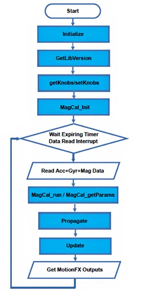
A flowchart of the demo software is also shown (Figure 5).
Figure 5: This flowchart illustrates the sequence of steps used by the MotionFX demo code in Listing 1 to extract data from STMicroelectronics’ X-NUCLEO-IKS01A2 expansion board and fuse it into a 3D spatial orientation. (Image source: STMicroelectronics)
Note that gyroscope data can drift, which can degrade the estimation of 3D spatial orientation. The MotionFX software can compensate for this degradation by using magnetometer data, which provides absolute orientation information. At the same time, magnetometers do not produce heading data at high rates and they suffer from magnetic disturbances, but gyroscope data can compensate for these magnetometer weaknesses.
The MotionFX software’s 9-axis sensor fusion calculations use data from the accelerometer, gyroscope, and magnetometer to provide absolute orientation in 3D space, including heading (relative to magnetic north).
The MotionFX software’s 6-axis sensor fusion calculations only use accelerometer and gyroscope data. This operational level has lower computational requirements and does not provide information about absolute orientation, but the routines run faster than the 9-axis routines. 6-axis sensor fusion is suitable for measuring fast movements, such as for gaming or for stationary robots, and can also be used when absolute orientation is not necessary.
Conclusion
IMUs are quite useful in embedded applications for providing location and heading information by themselves. They are also useful when used to augment GNSS receiver information when even higher precision or faster update rates are required. However, incorporating an IMU into an embedded system requires a significant amount of software, which IMU providers frequently supply to aid in the real-world application of these devices.
1. Introduction
INS is one of the important means for realizing vehicle positioning. It uses dead reckoning technology, based on IMU data, to compute the vehicle position information. SINS functions are a group of nonlinear equations. The position error, calculated based on inertial sensor data, includes two aspects, sensor measurement error and calculation error. When the IMU is confirmed, the position calculation method will directly affect the position estimation error. The nonlinear SINS functions should not cause divergent position error [1,2,3].
Today, deep learning is widely used in various fields, such as image processing, semantic understanding, speech processing, and data processing [4,5,6,7,8,9,10]. In recent years, deep learning has also been popular in the inertial navigation field [11]. Deep learning methods, like LSTM network and recurrent neural networks (RNN), have many advantages over forward networks for nonlinear system modeling [12,13]. The nonlinear autoregressive neural network is combined with an Unscented Kalman Filter (UKF) with external inputs to improve the position and velocity precision of the INS/Global Navigation Satellite System (GNSS) during GNSS outages [14]. RNN is used to improve the UKF for estimating and compensating the random drift of inertial sensors in real time [15]. To overcome the problem caused by overrange inertial measurement data, the faster region-based convolutional neural network (RCNN) method is proposed to realize robust autonomous navigation [16]. To improve the navigation ability of inertial/GPS integrated navigation system, LSTM is used to improve the system’s error prediction ability [17]. LSTM is used to estimate the com-cop inclination angle during walking based on inertial sensors [18]. LSTM-RNN is also proposed to denoise the MEMS IMU output signals [19]. A number of studies have shown that the application of deep learning to the inertial navigation field brings about new vitality to inertial technology [20,21,22].
In this study, a method is proposed that uses LSTM to estimate the position information based on the IMU data and GPS position information. Aiming at the structure of LSTM, the value range of LSTM hyperparameters is explored through the simulation. The results of LSTM estimation are compared with those computed with only SINS and those computed with a SINS/GPS loosely coupled KF during static positioning and dynamic positioning.
2. LSTM Net
LSTM takes sequences of information and uses recurrent mechanisms and gate techniques [23]. The structure, training/testing, and hyperparameters of LSTM are described in this section.
2.1. LSTM Net Structure
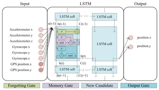
As shown in Figure 1, the rounded rectangle in the LSTM cell is the neural network layer of the LSTM [18,24]. The combination of a rounded rectangle and a multiplication operation is a gate. Gates are used to control the state of the LSTM cell. The repeating module in an LSTM cell contains four interacting layers: a forgetting gate layer, an input gate layer, a new candidate layer, and an output gate layer. In the LSTM net structure, the gate is realized by a sigmoid function:
σ(x)=1/1+e−x.
Figure 1. The LSTM net structure of inertial position estimation.
The forgetting gate layer is made by a sigmoid layer [25]:
f(t)=σ(Wf[h(t−1),x(t)]+bf).
The input gate layer decides what new information is going to be stored in the cell state. It has two steps. First, a sigmoid layer decides which values are to be updated. Next, a hyperbolic tangent function (tanh) layer creates a vector of new candidate values, C˜(t), that could be added to the state:
i(t)=σ(Wi[h(t−1),x(t)]+bi)
C˜(t)=tanh(WC[h(t−1),x(t)]+bC).
The new candidate layer is used to update the old cell state, C(t−1), into the new cell state C(t), as in the below equation:
C(t)=f(t)×C(t−1)+ii×C˜(t).
The output gate layer: the output is decided in this layer. First, it is going to be forgotten that the net decided to forget earlier. Then, we scale the new candidate values. Finally, we decide the output. The output is based on the cell states. The output computation is as in the below equations:
O(t)=σ(WO[h(t−1),x(t)]+bO)
h(t)=O(t)×tanh(C(t)).
As to the LSTM structure, the LSTM can use i(t) to decide when to keep or override information in memory cell C(t), and O(t) to decide when to access memory cell C(t) and when to prevent other units from being perturbed by C(t). The O(t) is the output information and the h(t) is the output about the LSTM structure.
Due to the forgetting gate in the structure, the LSTM net can realize the conditional prediction based on time. In another words, during the learning of a large amount of IMU data and GPS position data, the LSTM learns the position information characteristics related to time. The SINS computes the current inertial position information based on the last step. The SINS/GPS integrated navigation system using KF to estimate the position information is also based on the last step estimation at the current moment. Those processed can be regarded as a conditional prediction based on time. Therefore, we can use LSTM to estimate the position information based on IMU data and GPS position information. This means that the position information is defined as the features of IMU data. To learn the position features from IMU data, we also input the GPS position data to the LSTM net as the target.
2.2. LSTM Training and Testing Settings
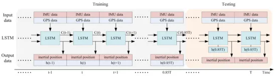
As shown in Figure 2, in this study, the training rate is 0.85. This means that 85% of the input dataset is the training set and the other 15% is the test set. Input and output size are based on the practical application of the LSTM.
Figure 2. Training and testing the LSTM to estimate position information.
As shown in Figure 1 and Figure 2, the input set includes two parts: IMU data, including three dimensions of gyroscope measurement data and three dimensions of accelerometer measurement data; and GPS data, including two dimensions of position information. The IMU data are the input of the LSTM, and the GPS data are the training target data. The output dataset includes two parts: the predicted inertial position, in two dimensions, and the output of the LSTM, with the number of dimensions based on the LSTM structure.
In LSTM, the purpose of net training is to optimize the weights and biases. The state activation function is the tanh, while the optimizer function is the adaptive moment estimation (Adam) stochastic gradient descent method with high convergence performance [18,26,27].
We use the root mean stand error (RMSE) to describe the training cost:
RMSE=1n∑ni=1(ypi−yi)2−−−−−−−−−−−−−−√,
where, ypi is the target GPS position data and yi is the inertial position predicted by LSTM.
2.3. Hyperparameters of LSTM
Hyperparameters need to be adjusted during LSTM training to make sure of the training cost in a confidence interval, including the time step, cell size, batch size, learning rate, and forgetting rate.
Time step: in LSTM, the purpose of net training is to optimize the weights and biases, to make sure the output errors are within a certain range. It is worth noting that the calculation of weights and biases is independent of the time step. In other words, the time step of LSTM can be set to any number. In this study, we expect that when the input IMU and target GPS data are at the same frequency, each frame of IMU data can be calculated to obtain the position information. Therefore, the time step in this study is 1.
Cell size: the hidden layer unit size, also called the hidden size. Cell size defines the deep degree of LSTM.
Batch size: also called mini-batch size. In the mini-batch gradient descent method, the data are divided into several batches and the parameters are updated according to the batches. In this way, the data in a batch jointly determine the direction of the gradient, so that the descent is not easy to determine, and the randomness is reduced. On the other hand, because the sample size of the batch is much smaller than the whole dataset, the computation burden will be reduced.
The learning rate and forgetting rate control the speed of adjusting weights and biases of neural network based on the loss gradient.
3. Simulation
To select appropriate hyperparameters such as the batch size, cell size, learning rate, and forgetting rate, we performed many simulations with different hyperparameters in this section.
3.1. Hyperparameter Evaluation
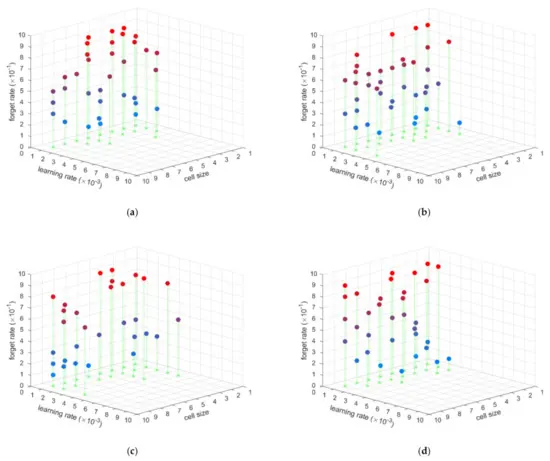
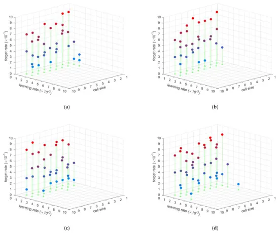
There are two simulation cases, static position estimation and dynamic position estimation. The IMU data used in the simulation are generated by the inertial simulator. The latitude and longitude of the initial location are set to 35° N and 108° E, respectively. The gyro constant drifts and random drifts are set to 0.02°/h and 0.001°/h, respectively. The accelerometer’s constant bias and random bias are 1 × 10⁻⁴ g and 1 × 10⁻⁵ g, respectively, where g is the local gravitation. In the static case, the simulation time is 60 s. In the dynamic case, the simulation time is 780 s, and the velocity is [1,1,0]T m/s. For each hyperparameter set, there are 100 training and testing events based on the simulated IMU data. We performed statistical tests on the hyperparameters used to train the LSTM to estimate the location based on the IMU data and GPS position information. The hyperparameters in the evaluation distribution point are the set that never cause overfitting or underfitting when training the LSTM to estimate the inertial position. They are recoded as shown in the following figures.
As each subgraph shows in Figure 3 and Figure 4, the hyperparameter evaluation distribution is similar when the batch size is different, and the hyperparameter evaluation distribution is also similar with different cell sizes and forgetting rates. However, different learning rates obviously affected the hyperparameter evaluation. Thus, the forgetting rate, cell size, and batch size have little influence on the LSTM used to estimate the position based IMU data. The important hyperparameter is the learning rate. From those simulations, when the learning rate is between 0.001 and 0.002, the LSTM is able to estimate the position based IMU data well. This hyperparameter evaluation applies to both static and dynamic situations. In another words, the static position estimation LSTM net and dynamic position estimation LSTM net have the same hyperparameter range. This means that an LSTM net with the same hyperparameters can be trained to estimate position based IMU data, no matter whether the conditions are static or dynamic.
Figure 3. The hyperparameter evaluation for static position estimation: (a) batch size is 5, (b) batch size is 10, (c) batch size is 15, (d) batch size is 20.
Figure 4. The hyperparameter evaluation for dynamic position estimation: (a) batch size is 5, (b) batch size is 10, (c) batch size is 15, (d) batch size is 20.
3.2. Position Estimation
In this section, the position information estimated by LSTM and the position information obtained by the inertial system functions are compared in static conditions and moving conditions. The uniform rectilinear motion data are simulated in the dynamic case.
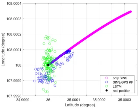
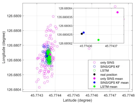
As shown in Figure 5, an LSTM net can fuse the IMU and GPS data to estimate the position information, as with the SINS/GPS loosely coupled based KF, in static simulation. Both an LSTM net and a loosely coupled KF-based system can restrain the divergence of only SINS. The position error STDs of only SINS, KF, and LSTM are 1.47 m, 0.88 m, and 0.77 m, respectively. The KF method computed position error STD is 59.86% for only SINSs, and the LSTM method estimated position error STD is 52.38% for only SINSs. The LSTM estimation position is more convergent than the KF method estimated.
Figure 5. Static position information of simulation.
The position error in the dynamic case is described by radial error. The radial error is defined by
where Le and λe are the estimation latitude and estimation longitude, respectively, and Lr and λr are the reference latitude and reference longitude, respectively. RN=Re/1−e2sin2L−−−−−−−−−√, RM=Re(1−e2)/(1−e2sin2L)3/2, Re is the ellipse major axis, and e is the ellipse eccentricity.
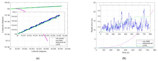
As shown in Figure 6a, LSTM net can fuse the IMU and GPS data to estimate the position information, like the SINS/GPS loosely coupled KF-based system, in a dynamic simulation. Both the LSTM net and the loosely coupled KF-based system can restrain the divergence of only SINS. As shown in Figure 6b, the biggest radial error of only SINS, KF method, and LSTM method are 21.21 m, 0.86 m, and 0.57 m, respectively. As Figure 6a,b shows, the position information obtained by only SINS has a nonlinear divergence error. The radial error of only SINS will continue to grow over time. However, the position error of KF and LSTM does not increase over time. The radial error of KF oscillates around 0. The radial error of LSTM is piecewise linear. Before 580 s, the position information estimated by LSTM has a linear divergence error. After 580 s, it becomes a constant error. LSTM can enforce constant error through “constant error carousels” within the forgetting gate during enough training steps [23]. The radial error of the LSTM estimation position accords with this conclusion.
Figure 6. (a) Dynamic position estimation of simulation; (b) dynamic position radial error of simulation.
As the simulation results show, the LSTM net can fuse the IMU and GPS data to estimate the position information and restrain the divergence error of only SINS, as with the SINS/GPS loosely coupled KF-based system.
4. Experiments
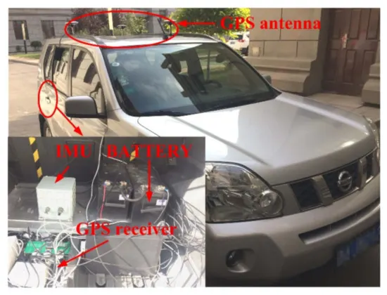
An experimental system was assembled to evaluate the proposed approach, as shown in Figure 7. The experimental equipment included an IMU, a GPS, and a power system on the vehicle. The IMU constituted a three-axis fiber-optic gyroscope with three accelerometers on each gyro-axis. The GPS was UR370 form UNICORE. The IMU, GPS receiver, and power system are in the vehicle trunk. The IMU is fixed on the vehicle via a steel plate that is parallel to the under panel of the vehicle. During the experiment, the IMU and GPS data were recoded. Both IMU data and GPS data included the GPS time. In this study, the GPS provided the position information target. The GPS data and IMU data were synchronized by their GPS times. There were two cases in the experiment, one static and the other dynamic. In static conditions, the vehicle stops 2 min. In dynamic conditions, the vehicle was driving in a uniform rectilinear motion along the road. The driving distance was 450 m and the driving speed was 2 km/s.
Figure 7. The experimental equipment.
As shown in Figure 8, an LSTM net can fuse the IMU and GPS data to estimate the position information, like the SINS/GPS loosely coupled KF-based system, in a static experiment. Both the LSTM net and loosely coupled KF-based system can restrain the divergence of only SINS. The position error STDs of only SINS, KF method, and LSTM method are 1.30 m, 0.33 m, and 0.30 m, respectively. The KF method computed position error STD is 25.38% for only SINSs, and the LSTM method computed position error STD is 23.08% for only SINSs. The LSTM estimation position is more convergent than the KF method estimated.
Figure 8. Static position of experiment.
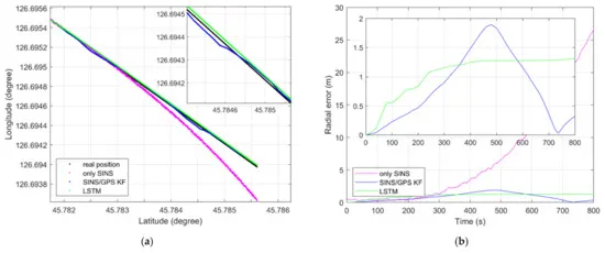
As shown in Figure 9a, an LSTM net can fuse the IMU data and GPS position information to estimate the position information, like the SINS/GPS loosely coupled KF-based system, in a dynamic experiment. Both the LSTM net and loosely coupled based KF can restrain the divergence of only SINS. As shown in Figure 9b, the largest radial error of only SINS, KF method, and LSTM method are 26.71 m, 1.89 m, and 1.31 m, respectively. As Figure 6a,b shows, the position information obtained by only SINS has nonlinear divergence error. The radial error of only SINS will continue to grow over time. However, the position error of KF method and LSTM method does not increase over time. The radial error of the KF method oscillates around 0. The radial error of LSTM method is piecewise linear. Before 450 s, the position information estimated by LSTM has linear divergence error. After 450 s, it becomes constant error. LSTM can enforce constant error through “constant error carousels” within the forgetting gate during enough training steps [23]. The radial error of the LSTM estimation position accords with this conclusion.
Figure 9. (a) Dynamic position estimation of experiment; (b) dynamic position radial error of experiment.
As the experimental results show, the LSTM net can fuse the IMU and GPS data to estimate the position information and restrain the divergence error of only SINS, like the SINS/GPS loosely coupled KF-based system.
5. Discussion
As the results of the simulations and experiments have shown, the effectiveness of the proposed method, using an LSTM net to fuse the IMU data and GPS to estimate the position information, has been proven in both static and dynamic conditions. Using the LSTM net to fuse IMU data and GPS position information can restrain the divergence of only SINS, like the SINS/GPS loosely coupled KF-based navigation system can.
The position error of only SINS includes sensor measurement error and calculation error. In this study, the simulation and experiment are based on the same IMU data and the same GPS position information. Thus, different position errors were found based on the calculation methods.
The model of position information calculation determines the character of the computational error. For the only SINS, as Equations (A3) and (A6) in Appendix A show, the position information and position error of only SINS are related to the inertial velocity computation and the inertial velocity error. The velocity information is integrated by geometric acceleration, and we get the position information by integrating the velocity information. The SINS functions and SINS error functions are nonlinear. The nonlinear error will accelerate the divergence of the position error through integration.
For the SINS/GPS loosely coupled KF-based navigation system, the system fusion the GPS position information and position, velocity and attitude information computed by only SINS, as Equations (A7) to (A9) in Appendix A show. The position information computed by only SINS diverges over time. The GPS position computing is without integral, so that GPS position information has almost no drift. Thus, based on KF, GPS position information can restrain the divergence of only SINS.
However, as Figure 2 shows, the IMU data are directly fused with GPS position information, without an inertial computer. Thus, there is no accumulation of error due to integration in the proposed method. As Equation (6) shows, the relationship between LSTM input information and LSTM output information is linear. The linear parameters are WO and bC. For a trained LSTM net, the structural parameters are constant. The error of LSTM estimation position is dependent on the parameters. The LSTM structure determines that the error of LSTM estimation position is linear. It is well known that suppression of linear error is easier than suppression of nonlinear error. Therefore, the LSTM position estimation method, which only produces linear error, makes the application of inertia information more convenient.
Both the KF method and the LSTM method can fuse GPS and an inertial sensor to restrain the error divergence of only SINS. There are some differences between the KF method and the LSTM method. For the KF information fusion method, it is a “white box.” It is applicable to the same navigation systems with the same system equation and same measurement equation. The system function and fusion function are definite. The system noise and measurement noise must be Gaussian white noise. With the same initial value, the position computed by the KF method is the same in every time. For the LSTM information fusion method, it is a “black box.” It is not required to give the specific equations of the system. The trained LSTM method model is only applicable to the system that provides the training and testing data. The LSTM output is based on the gate threshold value and the training cost function. There are no specific requirements for system noise or measurement noise. With the LSTM information fusion method, the position estimation output is different even with the same hyperparameters in every time. The outputs are distributed in an accuracy range.
6. Conclusions
In this study, we proposed a method using an LSTM net to estimate position information based on IMU data and GPS position information, because of its “memory” layer. Simulation and experimental results have shown that the proposed method is effective. The range of LSTM hyperparameters is explored through simulations. The LSTM information fusion method can restrain the position divergence of only SINS. In simulations, the LSTM method computed position error STD is 52.38% of only SINSs. The biggest simulation radial error estimated by the LSTM method is 0.57 m. In the experiments, the LSTM method computed position error STD at 23.08% for only SINSs. The biggest experimental radial error the LSTM method estimated was 1.31 m.
The trained LSTM fusion model is not applicable to all IMUs. It is only applicable to the IMU which provides the training data. The LSTM fusion method is used to estimate position information based on IMU data and GPS position, which only produces linear error, which makes the subsequent application of navigation information more convenient.
All in all, the trained LSTM is a dependable fusion method for combining IMU data and GPS position information to estimate position.
Author Contributions
Conceptualization, methodology, investigation, software, data curation, and visualization, X.G.; validation and formal analysis, X.G. and P.L.; resources, Y.G. and G.L.; writing—original draft preparation, X.G.; writing—review and editing, X.G. and P.L.; supervision, project administration, and funding acquisition, Y.G. All authors have read and agreed to the published version of the manuscript.
Funding
This research was funded by the National Natural Science Foundation of China, grant number 61803118; a Special Project of Chongqing Technology Innovation and Application Development, grant number Cstc2019jscx-Msxmx0423; and the Science and Technology Research Program of Chongqing Municipal Education Commission, grant number KJZD-K201804701.
Institutional Review Board Statement
Not applicable.
Informed Consent Statement
Not applicable.
Data Availability Statement
The data presented in this study are available on request from the corresponding author. The data are not publicly available due to ethics.
Acknowledgments
The authors would like to thank Shutong Li, Fan Zhang, and Yunlong Sun for helping with the experiments.
Conflicts of Interest
The authors declare no conflict of interest.
Appendix A
IMU data are computed into positioning/navigation information by a SINS algorithm [1]. The pose, velocity, and position information updating functions are shown below:
Cnb˙=Cnb(ωbib×)−(ωnin×)Cnb,
where ωbib is the IMU measurement angular velocity and ωnin is the rotation of navigation coordinate relative to the inertial coordinates.
vn˙=Cnbfbsb−(2ωnie+ωnen)×vn+gn,
where vn˙ is the geometric acceleration of the vehicle in the navigation coordinate system. fbsb is the IMU measurement accelerated velocity, while gn is the equatorial gravitation. −(2ωnie+ωnen)×vn is the harmful acceleration. Equation (A2) is called the inertial navigation specific force equation. We can get the velocity information by integrating vn˙ once, and the position information by integrating vn˙ twice. This is the base equation of the SINS algorithm:
p˙=Mpvvn,
where Mpv=⎡⎣⎢0secL/RNh01/RMh00001⎤⎦⎥.
In the navigation coordinates, the position error equations in dynamic conditions are as follows:
ϕ˙=Maaϕ+Mavδvn+Mapδp−Cnbεb,
where Maa=−(ωnin×)=⎡⎣⎢0−ωU−vEtanL/RNhωN+vE/RNhωU+vEtanL/RNh0vN/RMh−ωN−vE/RNh−vE/RNh0⎤⎦⎥, Mav=⎡⎣⎢01/RNhtanL/RNh−1/RMh00000⎤⎦⎥, Map=⎡⎣⎢⎢0−ωiesinLωiecosL+vEsec2L/RNh000vN/R2Mh−vE/R2Nh−vEtanL/R2Nh⎤⎦⎥⎥, where L, λ, and h denote the local latitude, longitude, and height, respectively; v defines the body velocity vector; ϕ describes the body pose errors; ε is the constant gyroscope drifts; the subscripts E, N and U denote the projection on the east, north, and up axes of the local coordinates, respectively. RNh=RN+h, RMh=RM+h, RN=Re/1−e2sin2L−−−−−−−−−√, and RM=Re(1−e2)/(1−e2sin2L)3/2, where Re is the ellipse major axis and e is the ellipse eccentricity.
The velocity error equations in the dynamic condition are as follows:
δv˙n=Mvaϕ+Mvvδvn+Mvpδp+Cnb∇b,
where Mvp=⎡⎣⎢⎢2(vNωN+vUωU)+vEvNsec2L/RNh−vE(2ωN+vEsec2L/RNh)2ωUvE+gesin2L(β−4β1cos2L)000vE(vU−vNtanL)/R2NhvEvN/R2Mh+v2EtanL/R2Nh−v2E/R2Mh−v2N/R2Nh+β2⎤⎦⎥⎥,
where ∇ denotes the accelerometer zero biases, f is the specific force, and β is the gravitation flattening, with β≈1/188.6, β1≈1/8(2βf+f2), and β2≈3.08×10⁻⁶s−2.
The position error equations in the dynamic condition are as follows:
δp˙=Mpvδvn+Mppδp,
where Mpp=⎡⎣⎢⎢0vEsecLtanL/RNh01/RMh00−vN/R2Mh−vEsecL/R2Nh0⎤⎦⎥⎥.
SINS information and GPS information can be fused by a KF [28]. For the loosely coupled method, the state vector is X=[δp,δvn,ϕ,∇b,εb]T and the system equation is
X˙=FX+GW,
where, F is the system matrix, G is the system noise matrix, and W is the system noise.
where, H is the system measurement matrix, V=[NnNe]T is the measurement noise, and Nn and Ne are the GPS measurement noise of North position and East position, respectively.
H=[R00RcosL013×2].
The KF includes a one-step state prediction equation, a state estimation equation, a filtering gain equation, a one-step prediction mean square error equation, and an estimated mean square error equation. They are listed below:
Xˆk+1,k=XFk+1,kXˆk
Xˆk+1=Xˆk+1,k+Kk(Zk−HkXˆk+1,k)
Kk+1=Pk+1,kHTk(HkPk+1,kHTk+Rk)−1
Pk+1,k=Fk+1,kPkFTk+1,k+Gk+1,kQkGTk+1,1
Pk+1=(I−KKHK)Pk(I−KKHK)T+KkRkKTk,
where, Xˆk+1,k denotes the prediction of the state vector from tk to tk+1, Xˆk denotes the prediction of the state vector at tk, Kk denotes filtering gain matrix, Pk+1,k denotes one-step estimated mean square error matrix from tk to tk+1, Pk denotes estiated mean square error matrix, Qk is system noise covariance matrix, and Rk denotes measurement noise covariance matrix.