Project 2 - EDA on Vehicle Insurance Customer Data
EDA on Vehicle Insurance Customer Data
In [1]:
# importing the required libraries

import pandas as pd
import numpy as np
import matplotlib.pyplot as plt
1. Adding the column names to both datasets while reading them:
In [2]:
## The "customer details" file is read and is given the column headings

table1 = pd.read_csv("customer_details.csv")
table1.columns=["Customer_id","Gender","Age","Driving_license_present","Region_Code","Previously_insured","Vehicle_age","Vehicle_damage"]
In [3]:
#To look at the customer details table
table1
Out[3]:
| Customer_id | Gender | Age | Driving_license_present | Region_Code | Previously_insured | Vehicle_age | Vehicle_damage | |
|---|---|---|---|---|---|---|---|---|
| 0 | 1.0 | Male | 44.0 | 1.0 | 28.0 | 0.0 | > 2 Years | Yes |
| 1 | 2.0 | Male | 76.0 | 1.0 | 3.0 | 0.0 | 1-2 Year | No |
| 2 | 3.0 | Male | 47.0 | 1.0 | 28.0 | 0.0 | > 2 Years | Yes |
| 3 | 4.0 | Male | 21.0 | 1.0 | 11.0 | 1.0 | < 1 Year | No |
| 4 | 5.0 | Female | 29.0 | 1.0 | 41.0 | 1.0 | < 1 Year | No |
| ... | ... | ... | ... | ... | ... | ... | ... | ... |
| 381104 | 381105.0 | Male | 74.0 | 1.0 | 26.0 | 1.0 | 1-2 Year | No |
| 381105 | 381106.0 | Male | 30.0 | 1.0 | 37.0 | 1.0 | < 1 Year | No |
| 381106 | 381107.0 | Male | 21.0 | 1.0 | 30.0 | 1.0 | < 1 Year | No |
| 381107 | 381108.0 | Female | 68.0 | 1.0 | 14.0 | 0.0 | > 2 Years | Yes |
| 381108 | 381109.0 | Male | 46.0 | 1.0 | 29.0 | 0.0 | 1-2 Year | No |
381109 rows × 8 columns
In [4]:
## The "customer_policy_details.csv file is read and the column names are given


table2 = pd.read_csv("customer_policy_details.csv")
table2.columns=["Customer_id", "Annual_premium", "Sales_Channel_Code", "Vintage", "Response" ]
In [5]:
#To look at the customer policy details table
table2
Out[5]:
| Customer_id | Annual_premium | Sales_Channel_Code | Vintage | Response | |
|---|---|---|---|---|---|
| 0 | 1.0 | 40454.0 | 26.0 | 217.0 | 1.0 |
| 1 | 2.0 | 33536.0 | 26.0 | 183.0 | 0.0 |
| 2 | 3.0 | 38294.0 | 26.0 | 27.0 | 1.0 |
| 3 | 4.0 | 28619.0 | 152.0 | 203.0 | 0.0 |
| 4 | 5.0 | 27496.0 | 152.0 | 39.0 | 0.0 |
| ... | ... | ... | ... | ... | ... |
| 381104 | 381105.0 | 30170.0 | 26.0 | 88.0 | 0.0 |
| 381105 | 381106.0 | 40016.0 | 152.0 | 131.0 | 0.0 |
| 381106 | 381107.0 | 35118.0 | 160.0 | 161.0 | 0.0 |
| 381107 | 381108.0 | 44617.0 | 124.0 | 74.0 | 0.0 |
| 381108 | 381109.0 | 41777.0 | 26.0 | 237.0 | 0.0 |
381109 rows × 5 columns
2. Checking and Cleaning Data Quality:
i.Scanning for Null values and cleaning if any present
In [6]:
# For table1

# Generating a summary of count of all the null values column wise for table 1

table1.isnull().sum()
Out[6]:
Customer_id                386
Gender                     368
Age                        368
Driving_license_present    393
Region_Code                392
Previously_insured         381
Vehicle_age                381
Vehicle_damage             407
dtype: int64
In [7]:
# Drop Null values for customer_id because central tendencies for id’s is not feasible

table1 = table1[~table1.Customer_id.isnull()].copy()


table1.isnull().sum()


table1
Out[7]:
| Customer_id | Gender | Age | Driving_license_present | Region_Code | Previously_insured | Vehicle_age | Vehicle_damage | |
|---|---|---|---|---|---|---|---|---|
| 0 | 1.0 | Male | 44.0 | 1.0 | 28.0 | 0.0 | > 2 Years | Yes |
| 1 | 2.0 | Male | 76.0 | 1.0 | 3.0 | 0.0 | 1-2 Year | No |
| 2 | 3.0 | Male | 47.0 | 1.0 | 28.0 | 0.0 | > 2 Years | Yes |
| 3 | 4.0 | Male | 21.0 | 1.0 | 11.0 | 1.0 | < 1 Year | No |
| 4 | 5.0 | Female | 29.0 | 1.0 | 41.0 | 1.0 | < 1 Year | No |
| ... | ... | ... | ... | ... | ... | ... | ... | ... |
| 381104 | 381105.0 | Male | 74.0 | 1.0 | 26.0 | 1.0 | 1-2 Year | No |
| 381105 | 381106.0 | Male | 30.0 | 1.0 | 37.0 | 1.0 | < 1 Year | No |
| 381106 | 381107.0 | Male | 21.0 | 1.0 | 30.0 | 1.0 | < 1 Year | No |
| 381107 | 381108.0 | Female | 68.0 | 1.0 | 14.0 | 0.0 | > 2 Years | Yes |
| 381108 | 381109.0 | Male | 46.0 | 1.0 | 29.0 | 0.0 | 1-2 Year | No |
380723 rows × 8 columns
In [8]:
# Replace all null values for numeric columns by mean for table 1

#numeric data
age_mean = table1['Age'].mean()
table1['Age'].fillna(value=age_mean,inplace=True)

region_mean = table1['Region_Code'].mean()
table1['Region_Code'].fillna(value=region_mean,inplace=True)
In [10]:
table1
Out[10]:
| Customer_id | Gender | Age | Driving_license_present | Region_Code | Previously_insured | Vehicle_age | Vehicle_damage | |
|---|---|---|---|---|---|---|---|---|
| 0 | 1.0 | Male | 44.0 | 1.0 | 28.0 | 0.0 | > 2 Years | Yes |
| 1 | 2.0 | Male | 76.0 | 1.0 | 3.0 | 0.0 | 1-2 Year | No |
| 2 | 3.0 | Male | 47.0 | 1.0 | 28.0 | 0.0 | > 2 Years | Yes |
| 3 | 4.0 | Male | 21.0 | 1.0 | 11.0 | 1.0 | < 1 Year | No |
| 4 | 5.0 | Female | 29.0 | 1.0 | 41.0 | 1.0 | < 1 Year | No |
| ... | ... | ... | ... | ... | ... | ... | ... | ... |
| 381104 | 381105.0 | Male | 74.0 | 1.0 | 26.0 | 1.0 | 1-2 Year | No |
| 381105 | 381106.0 | Male | 30.0 | 1.0 | 37.0 | 1.0 | < 1 Year | No |
| 381106 | 381107.0 | Male | 21.0 | 1.0 | 30.0 | 1.0 | < 1 Year | No |
| 381107 | 381108.0 | Female | 68.0 | 1.0 | 14.0 | 0.0 | > 2 Years | Yes |
| 381108 | 381109.0 | Male | 46.0 | 1.0 | 29.0 | 0.0 | 1-2 Year | No |
380723 rows × 8 columns
In [11]:
# Replace all null values for Categorical value by mode for table 1

#categorical data

gender_mode=table1.Gender.mode()[0]
table1.Gender.fillna(gender_mode,inplace=True)

driving_license_present_mode=table1.Driving_license_present.mode()[0]
table1.Driving_license_present.fillna(driving_license_present_mode,inplace=True)

previously_insured_mode=table1.Previously_insured.mode()[0]
table1.Previously_insured.fillna(previously_insured_mode,inplace=True)

vehicle_damage_mode=table1.Vehicle_damage.mode()[0]
table1.Vehicle_damage.fillna(vehicle_damage_mode,inplace=True)

vehicle_age_mode=table1.Vehicle_age.mode()[0]
table1.Vehicle_age.fillna(vehicle_age_mode,inplace=True)


table1.isnull().sum()


table1.describe()
Out[11]:
| Customer_id | Age | Driving_license_present | Region_Code | Previously_insured | |
|---|---|---|---|---|---|
| count | 380723.000000 | 380723.000000 | 380723.000000 | 380723.000000 | 380723.000000 |
| mean | 190548.776244 | 38.822788 | 0.997870 | 26.389436 | 0.457800 |
| std | 110016.805160 | 15.504826 | 0.046105 | 13.223671 | 0.498217 |
| min | 1.000000 | 20.000000 | 0.000000 | 0.000000 | 0.000000 |
| 25% | 95269.500000 | 25.000000 | 1.000000 | 15.000000 | 0.000000 |
| 50% | 190543.000000 | 36.000000 | 1.000000 | 28.000000 | 0.000000 |
| 75% | 285822.500000 | 49.000000 | 1.000000 | 35.000000 | 1.000000 |
| max | 381109.000000 | 85.000000 | 1.000000 | 52.000000 | 1.000000 |
In [12]:
# # For table2:
# Generating a summary of count of all the null values column wise

table2.isnull().sum()
Out[12]:
Customer_id           387
Annual_premium        346
Sales_Channel_Code    400
Vintage               388
Response              361
dtype: int64
In [13]:
# Drop Null values for customer_id because central tendencies for id’s is not feasible

table2 = table2[~table2.Customer_id.isnull()].copy()

table2.isnull().sum()
Out[13]:
Customer_id             0
Annual_premium        344
Sales_Channel_Code    400
Vintage               388
Response              361
dtype: int64
In [14]:
# Replace all null values for numeric columns by mean for table 2

#numeric data
annual_mean = table2['Annual_premium'].mean()
table2['Annual_premium'].fillna(value=annual_mean,inplace=True)

sales_channel_mean = table2['Sales_Channel_Code'].mean()
table2['Sales_Channel_Code'].fillna(value=sales_channel_mean,inplace=True)

vintage_mean = table2['Vintage'].mean()
table2['Vintage'].fillna(value=vintage_mean,inplace=True)
In [15]:
table2
Out[15]:
| Customer_id | Annual_premium | Sales_Channel_Code | Vintage | Response | |
|---|---|---|---|---|---|
| 0 | 1.0 | 40454.0 | 26.0 | 217.0 | 1.0 |
| 1 | 2.0 | 33536.0 | 26.0 | 183.0 | 0.0 |
| 2 | 3.0 | 38294.0 | 26.0 | 27.0 | 1.0 |
| 3 | 4.0 | 28619.0 | 152.0 | 203.0 | 0.0 |
| 4 | 5.0 | 27496.0 | 152.0 | 39.0 | 0.0 |
| ... | ... | ... | ... | ... | ... |
| 381104 | 381105.0 | 30170.0 | 26.0 | 88.0 | 0.0 |
| 381105 | 381106.0 | 40016.0 | 152.0 | 131.0 | 0.0 |
| 381106 | 381107.0 | 35118.0 | 160.0 | 161.0 | 0.0 |
| 381107 | 381108.0 | 44617.0 | 124.0 | 74.0 | 0.0 |
| 381108 | 381109.0 | 41777.0 | 26.0 | 237.0 | 0.0 |
380722 rows × 5 columns
In [16]:
# Replace all null values for Categorical value by mode for table 2

#categorical data

response_mode=table2.Response.mode()[0]
table2.Response.fillna(response_mode,inplace=True)


table2.isnull().sum()


table2.describe()
Out[16]:
| Customer_id | Annual_premium | Sales_Channel_Code | Vintage | Response | |
|---|---|---|---|---|---|
| count | 380722.000000 | 380722.000000 | 380722.000000 | 380722.000000 | 380722.000000 |
| mean | 190547.491663 | 30563.999774 | 112.036687 | 154.347192 | 0.122410 |
| std | 110013.824148 | 17190.147550 | 54.177046 | 83.628096 | 0.327759 |
| min | 1.000000 | 2630.000000 | 1.000000 | 10.000000 | 0.000000 |
| 25% | 95276.250000 | 24416.000000 | 29.000000 | 82.000000 | 0.000000 |
| 50% | 190536.500000 | 31656.000000 | 131.000000 | 154.000000 | 0.000000 |
| 75% | 285818.750000 | 39391.750000 | 152.000000 | 227.000000 | 0.000000 |
| max | 381109.000000 | 540165.000000 | 163.000000 | 299.000000 | 1.000000 |
Outliers detection For table1
In [17]:
# Age Outliers detection

x= table1.describe()["Age"]

IQR_age= x["75%"]-x["25%"]

table1[table1["Age"]<x["25%"]-1.5*IQR_age]

table1[table1["Age"]>x["75%"]+1.5*IQR_age]


# Region Code Outlier detection

y= table1.describe()["Region_Code"]

IQR_rc= y["75%"]-y["25%"]

table1[table1["Region_Code"]<x["25%"]-1.5*IQR_rc]

table1[table1["Region_Code"]>x["75%"]+1.5*IQR_rc]
Out[17]:
| Customer_id | Gender | Age | Driving_license_present | Region_Code | Previously_insured | Vehicle_age | Vehicle_damage |
|---|
In [18]:
table1
Out[18]:
| Customer_id | Gender | Age | Driving_license_present | Region_Code | Previously_insured | Vehicle_age | Vehicle_damage | |
|---|---|---|---|---|---|---|---|---|
| 0 | 1.0 | Male | 44.0 | 1.0 | 28.0 | 0.0 | > 2 Years | Yes |
| 1 | 2.0 | Male | 76.0 | 1.0 | 3.0 | 0.0 | 1-2 Year | No |
| 2 | 3.0 | Male | 47.0 | 1.0 | 28.0 | 0.0 | > 2 Years | Yes |
| 3 | 4.0 | Male | 21.0 | 1.0 | 11.0 | 1.0 | < 1 Year | No |
| 4 | 5.0 | Female | 29.0 | 1.0 | 41.0 | 1.0 | < 1 Year | No |
| ... | ... | ... | ... | ... | ... | ... | ... | ... |
| 381104 | 381105.0 | Male | 74.0 | 1.0 | 26.0 | 1.0 | 1-2 Year | No |
| 381105 | 381106.0 | Male | 30.0 | 1.0 | 37.0 | 1.0 | < 1 Year | No |
| 381106 | 381107.0 | Male | 21.0 | 1.0 | 30.0 | 1.0 | < 1 Year | No |
| 381107 | 381108.0 | Female | 68.0 | 1.0 | 14.0 | 0.0 | > 2 Years | Yes |
| 381108 | 381109.0 | Male | 46.0 | 1.0 | 29.0 | 0.0 | 1-2 Year | No |
380723 rows × 8 columns
Outliers detection For table2:
In [20]:
# Annual Premium outlier detection

x= table2.describe()["Annual_premium"]

IQR_ap= x["75%"]-x["25%"]

table2[table2["Annual_premium"]<x["25%"]-1.5*IQR_ap]

table2[table2["Annual_premium"]>x["75%"]+1.5*IQR_ap]

mean = table2["Annual_premium"].mean()
upper_outliers = table2["Annual_premium"]>x["75%"]+1.5*IQR_ap

mean
table2.loc[upper_outliers,"Annual_premium"]=np.nan
table2["Annual_premium"].fillna(mean,inplace=True)

table2[table2["Annual_premium"]>x["75%"]+1.5*IQR_ap]
Out[20]:
| Customer_id | Annual_premium | Sales_Channel_Code | Vintage | Response |
|---|
In [21]:
# Sales Channel Code Outlier detection

x= table2.describe()["Sales_Channel_Code"]

IQR_scc= x["75%"]-x["25%"]

table2[table2["Sales_Channel_Code"]<x["25%"]-1.5*IQR_scc]

table2[table2["Sales_Channel_Code"]>x["75%"]+1.5*IQR_scc]
Out[21]:
| Customer_id | Annual_premium | Sales_Channel_Code | Vintage | Response |
|---|
In [22]:
# Vintage Outlier Detection

x= table2.describe()["Vintage"]

IQR_v= x["75%"]-x["25%"]

table2[table2["Vintage"]<x["25%"]-1.5*IQR_v]


table2[table2["Vintage"]>x["75%"]+1.5*IQR_v]
Out[22]:
| Customer_id | Annual_premium | Sales_Channel_Code | Vintage | Response |
|---|
iii. Removing White spaces
In [23]:
table1.head()


table1['Vehicle_age'].str.replace(' ','')
table1['Gender'].str.replace(' ','')
table1['Vehicle_damage'].replace(' ','')
table1
Out[23]:
| Customer_id | Gender | Age | Driving_license_present | Region_Code | Previously_insured | Vehicle_age | Vehicle_damage | |
|---|---|---|---|---|---|---|---|---|
| 0 | 1.0 | Male | 44.0 | 1.0 | 28.0 | 0.0 | > 2 Years | Yes |
| 1 | 2.0 | Male | 76.0 | 1.0 | 3.0 | 0.0 | 1-2 Year | No |
| 2 | 3.0 | Male | 47.0 | 1.0 | 28.0 | 0.0 | > 2 Years | Yes |
| 3 | 4.0 | Male | 21.0 | 1.0 | 11.0 | 1.0 | < 1 Year | No |
| 4 | 5.0 | Female | 29.0 | 1.0 | 41.0 | 1.0 | < 1 Year | No |
| ... | ... | ... | ... | ... | ... | ... | ... | ... |
| 381104 | 381105.0 | Male | 74.0 | 1.0 | 26.0 | 1.0 | 1-2 Year | No |
| 381105 | 381106.0 | Male | 30.0 | 1.0 | 37.0 | 1.0 | < 1 Year | No |
| 381106 | 381107.0 | Male | 21.0 | 1.0 | 30.0 | 1.0 | < 1 Year | No |
| 381107 | 381108.0 | Female | 68.0 | 1.0 | 14.0 | 0.0 | > 2 Years | Yes |
| 381108 | 381109.0 | Male | 46.0 | 1.0 | 29.0 | 0.0 | 1-2 Year | No |
380723 rows × 8 columns
iv. case correction. Convert string values to uppercase
In [24]:
table1["Gender"]=table1["Gender"].str.upper()
table1["Vehicle_damage"]=table1["Vehicle_damage"].str.upper()

table1.sample(10)
Out[24]:
| Customer_id | Gender | Age | Driving_license_present | Region_Code | Previously_insured | Vehicle_age | Vehicle_damage | |
|---|---|---|---|---|---|---|---|---|
| 131046 | 131047.0 | MALE | 25.0 | 1.0 | 41.0 | 1.0 | < 1 Year | NO |
| 116643 | 116644.0 | MALE | 23.0 | 1.0 | 28.0 | 1.0 | < 1 Year | NO |
| 178081 | 178082.0 | FEMALE | 23.0 | 1.0 | 8.0 | 1.0 | < 1 Year | NO |
| 371603 | 371604.0 | FEMALE | 71.0 | 1.0 | 33.0 | 0.0 | 1-2 Year | YES |
| 238765 | 238766.0 | MALE | 65.0 | 1.0 | 28.0 | 0.0 | 1-2 Year | YES |
| 47911 | 47912.0 | MALE | 38.0 | 1.0 | 22.0 | 0.0 | 1-2 Year | YES |
| 313415 | 313416.0 | FEMALE | 24.0 | 1.0 | 8.0 | 1.0 | < 1 Year | NO |
| 79924 | 79925.0 | FEMALE | 25.0 | 1.0 | 21.0 | 1.0 | < 1 Year | NO |
| 358882 | 358883.0 | FEMALE | 46.0 | 1.0 | 22.0 | 0.0 | 1-2 Year | NO |
| 190166 | 190167.0 | FEMALE | 55.0 | 1.0 | 28.0 | 0.0 | 1-2 Year | YES |
v. Convert nominal data (categorical) into dummies
In [25]:
# for future modeling use if required


table1_d=pd.get_dummies(table1, columns=['Gender','Vehicle_damage','Driving_license_present','Previously_insured','Vehicle_age'])


table2_d=pd.get_dummies(table2,columns=['Response'])
vi. Droping Duplicates (duplicated rows)
In [26]:
table1.drop_duplicates(inplace=True)
table1_d.drop_duplicates(inplace=True) #table1 with the dummy columns


table2.drop_duplicates(inplace=True)
table2_d.drop_duplicates(inplace=True) #table2 with the dummy columns
3. Create a Master table for future use. Join the customer table and customer_policy table
In [27]:
# to get a master table using customer_id in both tables.


table_merge=pd.merge(table1,table2,on='Customer_id')


table_merge_d=pd.merge(table1_d,table2_d,on="Customer_id") #this is a merged table for the dummies table


table_merge


table_merge_d.describe()


table_merge.describe()
Out[27]:
| Customer_id | Age | Driving_license_present | Region_Code | Previously_insured | Annual_premium | Sales_Channel_Code | Vintage | Response | |
|---|---|---|---|---|---|---|---|---|---|
| count | 380336.000000 | 380336.000000 | 380336.000000 | 380336.000000 | 380336.000000 | 380336.000000 | 380336.000000 | 380336.000000 | 380336.000000 |
| mean | 190541.253954 | 38.822339 | 0.997868 | 26.389690 | 0.457811 | 29300.333246 | 112.037616 | 154.353300 | 0.122423 |
| std | 110013.789585 | 15.505135 | 0.046128 | 13.223789 | 0.498218 | 14532.972093 | 54.176953 | 83.630142 | 0.327775 |
| min | 1.000000 | 20.000000 | 0.000000 | 0.000000 | 0.000000 | 2630.000000 | 1.000000 | 10.000000 | 0.000000 |
| 25% | 95267.750000 | 25.000000 | 1.000000 | 15.000000 | 0.000000 | 24416.000000 | 29.000000 | 82.000000 | 0.000000 |
| 50% | 190524.500000 | 36.000000 | 1.000000 | 28.000000 | 0.000000 | 30949.000000 | 131.000000 | 154.000000 | 0.000000 |
| 75% | 285809.250000 | 49.000000 | 1.000000 | 35.000000 | 1.000000 | 38336.000000 | 152.000000 | 227.000000 | 0.000000 |
| max | 381109.000000 | 85.000000 | 1.000000 | 52.000000 | 1.000000 | 61854.000000 | 163.000000 | 299.000000 | 1.000000 |
4. Gaining insights from the data for future growth of the insurance company
In [28]:
# The following information are collected:

# i. Gender wise average annual premium: To find the gender who have taken the most policies from the company so we can
# find ways to further increase the number

table_merge.groupby('Gender')['Annual_premium'].mean()
Out[28]:
Gender
FEMALE    29273.474247
MALE      29323.099677
Name: Annual_premium, dtype: float64
In [29]:
# # ii. Age wise average annual premium: The result is plotted as a graph to get visualized result of the age distribution
# of the policy holder's average annual premium

age_plot= table_merge.groupby('Age')['Annual_premium'].mean()
age_plot.plot()
plt.show()


age_plot  #age wise average annual premium
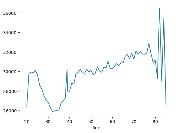
Out[29]:
Age
20.0    26342.073517
21.0    29751.791916
22.0    29946.848634
23.0    29838.344763
24.0    30125.557096
            ...
81.0    29287.910702
82.0    36480.586199
83.0    28995.818172
84.0    35440.818182
85.0    26637.454525
Name: Annual_premium, Length: 67, dtype: float64
In [31]:
#iii. Finding if the data is balanced between the two genders

print("Proportion of Males in data: ", table_merge_d[table_merge_d["Gender_MALE"]==1].shape[0]/table_merge_d.shape[0]*100)


print("Proportion Females in data:",table_merge_d[table_merge_d["Gender_FEMALE"]==1].shape[0]/table_merge_d.shape[0]*100)
Proportion of Males in data:  54.123459257077954
Proportion Females in data: 45.87654074292205
In [32]:
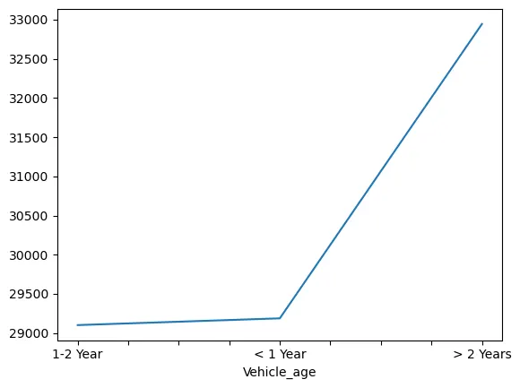
#iv. Vehicle age wise average annual premium.

table_merge.groupby('Vehicle_age')['Annual_premium'].mean()


vehicle_age_plot= table_merge.groupby('Vehicle_age')['Annual_premium'].mean()
vehicle_age_plot.plot()
plt.show()
5. Is there any relation between Person Age and annual premium?
In [33]:
# # Is there any relation between Person Age and annual premium?

n = table_merge["Age"].corr(table_merge["Annual_premium"])


if n<-0.5:
    print("Strong negative relationship")
elif n>0.5:
    print("Strong positive relationship")
elif n>-0.5 and n <0.5:
    print("There is no relationship")


table_merge.to_csv('table_merge.csv',index=False)
There is no relationship