Project 2 - EDA on Vehicle Insurance Customer Data
import pandas as pd
import numpy as np
import matplotlib.pyplot as plt
In [2]:
# add on data
df1 = pd.read_csv("customer_details.csv", encoding='ISO-8859-1')
df2 = pd.read_csv("customer_policy.csv", encoding='ISO-8859-1')
In [3]:
#Adding column name to customer Details-
col1=["Id","Gender","Age","Driving licence Active","regin code","Previously Insured","Vehical Age","Vehical Damage"]
df1.columns = col1
df1.head()
Out[3]:
| Id | Gender | Age | Driving licence Active | regin code | Previously Insured | Vehical Age | Vehical Damage | |
|---|---|---|---|---|---|---|---|---|
| 0 | 1 | Male | 44 | 1 | 28 | 0 | >2 Years | Yes |
| 1 | 2 | Male | 76 | 1 | 3 | 0 | 1-2 Years | No |
| 2 | 3 | Male | 47 | 1 | 28 | 0 | >2 Years | Yes |
| 3 | 4 | Male | 21 | 1 | 11 | 1 | <1 Years | No |
| 4 | 5 | Famele | 29 | 1 | 41 | 1 | <1 Years | No |
In [4]:
#Adding column to Coustomer policy details-
col2 = ["Id","Anaual Salary","Sale channel code","Vintage","Response"]
df2.columns=col2
df2.head()
Out[4]:
| Id | Anaual Salary | Sale channel code | Vintage | Response | |
|---|---|---|---|---|---|
| 0 | 1 | 40454 | 26 | 217 | 1 |
| 1 | 2 | 33536 | 26 | 183 | 0 |
| 2 | 3 | 38294 | 26 | 27 | 1 |
| 3 | 4 | 28619 | 152 | 203 | 0 |
| 4 | 5 | 27496 | 152 | 39 | 0 |
In [5]:
#Null Value cheaking
#coustomer Deatils
df1_n = df1.isnull()
for i in df1_n.columns.values.tolist():
print(i)
print(df1_n[i].value_counts())
print("")
Id
False    5
Name: Id, dtype: int64

Gender
False    5
Name: Gender, dtype: int64

Age
False    5
Name: Age, dtype: int64

Driving licence Active
False    5
Name: Driving licence Active, dtype: int64

regin code
False    5
Name: regin code, dtype: int64

Previously Insured
False    5
Name: Previously Insured, dtype: int64

Vehical Age
False    5
Name: Vehical Age, dtype: int64

Vehical Damage
False    5
Name: Vehical Damage, dtype: int64
In [6]:
# null value checking
#coustomer policy Deatils
df2_n = df2.isnull()
for i in df2_n.columns.values.tolist():
print(i)
print(df2_n[i].value_counts())
print("")
Id
False    5
Name: Id, dtype: int64

Anaual Salary
False    5
Name: Anaual Salary, dtype: int64

Sale channel code
False    5
Name: Sale channel code, dtype: int64

Vintage
False    5
Name: Vintage, dtype: int64

Response
False    5
Name: Response, dtype: int64
In [7]:
#-----------------------Dropping Null Values-----------------------
#coustomer Deatils
df1.dropna(subset=['Id'],axis = 0,inplace = True)
df1.reset_index(drop = True,inplace=True)
#-----------------------Dropping Null Values-----------------------
#coustomer Policy Deatils
df2.dropna(subset=['Id'],axis = 0,inplace = True)
df2.reset_index(drop = True,inplace=True)
#--------------------------Replacing all Null Values---------------
#Replacing the NaN value of age by its mean value
df1['Age'].fillna(df1['Age'].mean(),inplace=True)
##Replacing the NaN value of region code by its mean value
df1['regin code'].fillna(df1['regin code'].mean(),inplace=True)
df1.head()
Out[7]:
| Id | Gender | Age | Driving licence Active | regin code | Previously Insured | Vehical Age | Vehical Damage | |
|---|---|---|---|---|---|---|---|---|
| 0 | 1 | Male | 44 | 1 | 28 | 0 | >2 Years | Yes |
| 1 | 2 | Male | 76 | 1 | 3 | 0 | 1-2 Years | No |
| 2 | 3 | Male | 47 | 1 | 28 | 0 | >2 Years | Yes |
| 3 | 4 | Male | 21 | 1 | 11 | 1 | <1 Years | No |
| 4 | 5 | Famele | 29 | 1 | 41 | 1 | <1 Years | No |
In [8]:
#--------------------------Replacing all Null Values---------------
#Replacing the NaN value of age by its mean value
df2['Anaual Salary'].fillna(df2['Anaual Salary'].mean(),inplace=True)
##Replacing the NaN value of sale channel code by its mean value
df2['Sale channel code'].fillna(df2['Sale channel code'].mean(),inplace=True)
##Replacing the NaN value of vintage code by its mean value
df2['Vintage'].fillna(df2['Vintage'].mean(),inplace=True)
df2.head()
Out[8]:
| Id | Anaual Salary | Sale channel code | Vintage | Response | |
|---|---|---|---|---|---|
| 0 | 1 | 40454 | 26 | 217 | 1 |
| 1 | 2 | 33536 | 26 | 183 | 0 |
| 2 | 3 | 38294 | 26 | 27 | 1 |
| 3 | 4 | 28619 | 152 | 203 | 0 |
| 4 | 5 | 27496 | 152 | 39 | 0 |
In [9]:
#--------------------------Replacing Categorical Null Values by Mode---------------
#Replacing the NaN value of Driving licence Active by its mode value
df1['Driving licence Active'].fillna(df1['Driving licence Active'].mode()[0],inplace=True)
##Replacing the NaN value of Previously Insured by its mode value
df1['Previously Insured'].fillna(df1['Previously Insured'].mode()[0],inplace=True)
df1.head()
Out[9]:
| Id | Gender | Age | Driving licence Active | regin code | Previously Insured | Vehical Age | Vehical Damage | |
|---|---|---|---|---|---|---|---|---|
| 0 | 1 | Male | 44 | 1 | 28 | 0 | >2 Years | Yes |
| 1 | 2 | Male | 76 | 1 | 3 | 0 | 1-2 Years | No |
| 2 | 3 | Male | 47 | 1 | 28 | 0 | >2 Years | Yes |
| 3 | 4 | Male | 21 | 1 | 11 | 1 | <1 Years | No |
| 4 | 5 | Famele | 29 | 1 | 41 | 1 | <1 Years | No |
In [10]:
#--------------------------Replacing Categorical Null Values by Mode-----------
#Replacing the NaN value of Responce by its mode value
df2['Response'].fillna(df2['Response'].mode()[0],inplace=True)
df2.head()
Out[10]:
| Id | Anaual Salary | Sale channel code | Vintage | Response | |
|---|---|---|---|---|---|
| 0 | 1 | 40454 | 26 | 217 | 1 |
| 1 | 2 | 33536 | 26 | 183 | 0 |
| 2 | 3 | 38294 | 26 | 27 | 1 |
| 3 | 4 | 28619 | 152 | 203 | 0 |
| 4 | 5 | 27496 | 152 | 39 | 0 |
In [12]:
#----------------------------Visualisation of Outliers-------------
def plot_boxplot(df,ft):
df.boxplot(column=[ft])
plt.grid(False)
plt.show
plot_boxplot(df1,'Age')

In [13]:
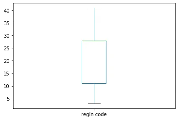
plot_boxplot(df1,'regin code')
In [14]:
#---------------------------------------------------IQR Method---------------------------------------------
#this function finds outliers if present by IQR method
def finding_out(df):
q1 = df.quantile(0.25)
q3=df.quantile(0.75)
iqr=q3-q1
outlier = df[((df<(q1-1.5*iqr)))|(df>(q3+1.5*iqr))]
return outlier
outliers = finding_out(df1['regin code'])
print("Number of outliers:",len(outliers))
print("Max Number of outliers:",outliers.max())
print("Minimum outlier value:",outliers.min())
Number of outliers: 0
Max Number of outliers: nan
Minimum outlier value: nan
In [15]:
#-------------------------------Finding Outliers for customer policy details----------------------------------
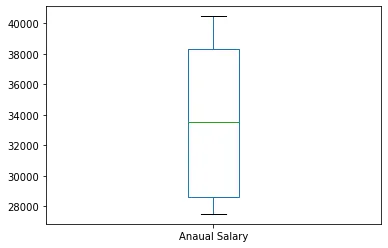
plot_boxplot(df2,'Anaual Salary')
In [16]:
plot_boxplot(df2,'Sale channel code')

In [17]:
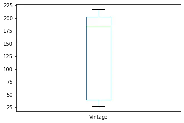
plot_boxplot(df2,'Vintage')
In [18]:
#-----------------------The summary of the Outliers-------------------------------------------
print("For Annual Salary")
outliers = finding_out(df2['Anaual Salary'])
print("Number of outliers:",len(outliers))
print("Max Number of outliers:",outliers.max())
print("Minimum outlier value:",outliers.min())
print('-**-'*16)
print("For sales channel code")
outliers = finding_out(df2['Sale channel code'])
print("Number of outliers:",len(outliers))
print("Max Number of outliers:",outliers.max())
print("Minimum outlier value:",outliers.min())
print('-**-'*16)
print("For Vintage")
outliers = finding_out(df2['Vintage'])
print("Number of outliers:",len(outliers))
print("Max Number of outliers:",outliers.max())
print("Minimum outlier value:",outliers.min())
print('-**-'*16)
For Annual Salary
Number of outliers: 0
Max Number of outliers: nan
Minimum outlier value: nan
-**--**--**--**--**--**--**--**--**--**--**--**--**--**--**--**-
For sales channel code
Number of outliers: 0
Max Number of outliers: nan
Minimum outlier value: nan
-**--**--**--**--**--**--**--**--**--**--**--**--**--**--**--**-
For Vintage
Number of outliers: 0
Max Number of outliers: nan
Minimum outlier value: nan
-**--**--**--**--**--**--**--**--**--**--**--**--**--**--**--**-
In [19]:
#---------------------------------------Replacing the outliers with mean values_________________________________
def replace(df):
q1 = df.quantile(0.25)
q3=df.quantile(0.75)
iqr=q3-q1
upper = df[~(df>(q3+1.5*iqr))].max()
lower = df[~(df>(q3+1.5*iqr))].min()
return df
replace(df2['Anaual Salary'])
Out[19]:
0    40454
1    33536
2    38294
3    28619
4    27496
Name: Anaual Salary, dtype: int64
In [20]:
#--------------------------------------Remove White Spaces---------------------------------------------
df1.apply(lambda x:x.str.strip() if x.dtype == 'object'else x)
Out[20]:
| Id | Gender | Age | Driving licence Active | regin code | Previously Insured | Vehical Age | Vehical Damage | |
|---|---|---|---|---|---|---|---|---|
| 0 | 1 | Male | 44 | 1 | 28 | 0 | >2 Years | Yes |
| 1 | 2 | Male | 76 | 1 | 3 | 0 | 1-2 Years | No |
| 2 | 3 | Male | 47 | 1 | 28 | 0 | >2 Years | Yes |
| 3 | 4 | Male | 21 | 1 | 11 | 1 | <1 Years | No |
| 4 | 5 | Famele | 29 | 1 | 41 | 1 | <1 Years | No |
In [21]:
#--------------------------------------Case Correctio------------------------------------------
df1.apply(lambda x:x.str.upper() if x.dtype == 'object'else x)
Out[21]:
| Id | Gender | Age | Driving licence Active | regin code | Previously Insured | Vehical Age | Vehical Damage | |
|---|---|---|---|---|---|---|---|---|
| 0 | 1 | MALE | 44 | 1 | 28 | 0 | >2 YEARS | YES |
| 1 | 2 | MALE | 76 | 1 | 3 | 0 | 1-2 YEARS | NO |
| 2 | 3 | MALE | 47 | 1 | 28 | 0 | >2 YEARS | YES |
| 3 | 4 | MALE | 21 | 1 | 11 | 1 | <1 YEARS | NO |
| 4 | 5 | FAMELE | 29 | 1 | 41 | 1 | <1 YEARS | NO |
In [22]:
#------------------------------------convert nominal data into dummy variables---------------------------------------
dummy_variable_1 = pd.get_dummies(df1['Vehical Damage'])
dummy_variable_1.rename(columns={'No':'vehicale-damage-No','Yes':'vehicle-damage-Yes'},inplace = True)
dummy_variable_1.head()
Out[22]:
| vehicale-damage-No | vehicle-damage-Yes | |
|---|---|---|
| 0 | 0 | 1 |
| 1 | 1 | 0 |
| 2 | 0 | 1 |
| 3 | 1 | 0 |
| 4 | 1 | 0 |
In [24]:
# Merging The Data Set
master_data = pd.merge(df1,df2,on='Id')
master_data
Out[24]:
| Id | Gender | Age | Driving licence Active | regin code | Previously Insured | Vehical Age | Vehical Damage | Anaual Salary | Sale channel code | Vintage | Response | |
|---|---|---|---|---|---|---|---|---|---|---|---|---|
| 0 | 1 | Male | 44 | 1 | 28 | 0 | >2 Years | Yes | 40454 | 26 | 217 | 1 |
| 1 | 2 | Male | 76 | 1 | 3 | 0 | 1-2 Years | No | 33536 | 26 | 183 | 0 |
| 2 | 3 | Male | 47 | 1 | 28 | 0 | >2 Years | Yes | 38294 | 26 | 27 | 1 |
| 3 | 4 | Male | 21 | 1 | 11 | 1 | <1 Years | No | 28619 | 152 | 203 | 0 |
| 4 | 5 | Famele | 29 | 1 | 41 | 1 | <1 Years | No | 27496 | 152 | 39 | 0 |
In [25]:
#Getting Required Data for decisions
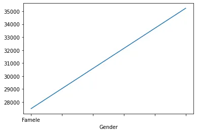
all_data = master_data.groupby('Gender')['Anaual Salary'].mean()
all_data
Out[25]:
Gender
Famele    27496.00
Male      35225.75
Name: Anaual Salary, dtype: float64
In [26]:
all_data.plot()
Out[26]:
<AxesSubplot:xlabel='Gender'>
In [27]:
all_data.plot.bar(title='Gender vs Annual Salary')
Out[27]:
<AxesSubplot:title={'center':'Gender vs Annual Salary'}, xlabel='Gender'>

In [28]:
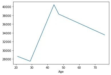
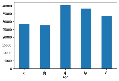
#-----------------------------------------Age wise average annual premium-----------------------------------
age_data =master_data.groupby('Age')['Anaual Salary'].mean()
age_data
Out[28]:
Age
21    28619.0
29    27496.0
44    40454.0
47    38294.0
76    33536.0
Name: Anaual Salary, dtype: float64
In [29]:
age_data.plot()
Out[29]:
<AxesSubplot:xlabel='Age'>
In [30]:
age_data.plot.bar()
Out[30]:
<AxesSubplot:xlabel='Age'>
In [31]:
#------------------------------------------------Checking Balanced Between gender or no---------------------------
master_data.groupby('Gender').count()
Out[31]:
| Id | Age | Driving licence Active | regin code | Previously Insured | Vehical Age | Vehical Damage | Anaual Salary | Sale channel code | Vintage | Response | |
|---|---|---|---|---|---|---|---|---|---|---|---|
| Gender | |||||||||||
| Famele | 1 | 1 | 1 | 1 | 1 | 1 | 1 | 1 | 1 | 1 | 1 |
| Male | 4 | 4 | 4 | 4 | 4 | 4 | 4 | 4 | 4 | 4 | 4 |
In [32]:
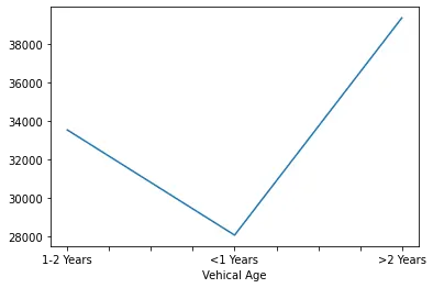
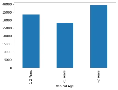
#------------------------------------------------Vehical age wise average salary---------------------------------------
vehical_age =master_data.groupby('Vehical Age')['Anaual Salary'].mean()
vehical_age
Out[32]:
Vehical Age
1-2 Years    33536.0
<1 Years     28057.5
>2 Years     39374.0
Name: Anaual Salary, dtype: float64
In [33]:
vehical_age.plot()
Out[33]:
<AxesSubplot:xlabel='Vehical Age'>
In [34]:
vehical_age.plot.bar()
Out[34]:
<AxesSubplot:xlabel='Vehical Age'>
In [35]:
#Correlation Between age and annual premuim
master_data['Age'].corr(master_data['Anaual Salary'])
Out[35]:
0.4515226822803064
In [36]:
master_data[['Age','Anaual Salary']].corr()
Out[36]:
| Age | Anaual Salary | |
|---|---|---|
| Age | 1.000000 | 0.451523 |
| Anaual Salary | 0.451523 | 1.000000 |