Project 2 - EDA on Vehicle Insurance Customer Data
import numpy as np
import pandas as pd
from matplotlib import pyplot as plt
import seaborn as sns
customerD = pd.read_csv("customer_details.csv")
customerPD = pd.read_csv("customer_policy_details.csv")
1. Add the column names to both datasets:
i. Column Name for customer details table
customerD.columns
Index(['0', '1', '2', '3', '4', '5', '6', '7'], dtype='object')
customerD.rename(columns={'0':'customer_id', '1':'Gender', '2':'age', '3':'driving licence present', '4':'region code','5':'previously insured', '6':'vehicle age', '7':'vehicle damage'})
| customer_id | Gender | age | driving licence present | region code | previously insured | vehicle age | vehicle damage | |
|---|---|---|---|---|---|---|---|---|
| 0 | 1.0 | Male | 44.0 | 1.0 | 28.0 | 0.0 | > 2 Years | Yes |
| 1 | 2.0 | Male | 76.0 | 1.0 | 3.0 | 0.0 | 1-2 Year | No |
| 2 | 3.0 | Male | 47.0 | 1.0 | 28.0 | 0.0 | > 2 Years | Yes |
| 3 | 4.0 | Male | 21.0 | 1.0 | 11.0 | 1.0 | < 1 Year | No |
| 4 | 5.0 | Female | 29.0 | 1.0 | 41.0 | 1.0 | < 1 Year | No |
| ... | ... | ... | ... | ... | ... | ... | ... | ... |
| 381104 | 381105.0 | Male | 74.0 | 1.0 | 26.0 | 1.0 | 1-2 Year | No |
| 381105 | 381106.0 | Male | 30.0 | 1.0 | 37.0 | 1.0 | < 1 Year | No |
| 381106 | 381107.0 | Male | 21.0 | 1.0 | 30.0 | 1.0 | < 1 Year | No |
| 381107 | 381108.0 | Female | 68.0 | 1.0 | 14.0 | 0.0 | > 2 Years | Yes |
| 381108 | 381109.0 | Male | 46.0 | 1.0 | 29.0 | 0.0 | 1-2 Year | No |
381109 rows × 8 columns
customerD=customerD.rename(columns={'0':'customer_id', '1':'Gender', '2':'age', '3':'driving licence present', '4':'region code','5':'previously insured', '6':'vehicle age', '7':'vehicle damage'})
customerD.head(2)
| customer_id | Gender | age | driving licence present | region code | previously insured | vehicle age | vehicle damage | |
|---|---|---|---|---|---|---|---|---|
| 0 | 1.0 | Male | 44.0 | 1.0 | 28.0 | 0.0 | > 2 Years | Yes |
| 1 | 2.0 | Male | 76.0 | 1.0 | 3.0 | 0.0 | 1-2 Year | No |
customerD.columns
Index(['customer_id', 'Gender', 'age', 'driving licence present',
       'region code', 'previously insured', 'vehicle age', 'vehicle damage'],
      dtype='object')
ii. Column Name for customer_policy table
customerPD.columns
Index(['0', '1', '2', '3', '4'], dtype='object')
customerPD.rename(columns={'0':'customer_id', '1':'annual premium (in Rs)', '2':'sales channel code', '3':'vintage','4':'response'})
| customer_id | annual premium (in Rs) | sales channel code | vintage | response | |
|---|---|---|---|---|---|
| 0 | 1.0 | 40454.0 | 26.0 | 217.0 | 1.0 |
| 1 | 2.0 | 33536.0 | 26.0 | 183.0 | 0.0 |
| 2 | 3.0 | 38294.0 | 26.0 | 27.0 | 1.0 |
| 3 | 4.0 | 28619.0 | 152.0 | 203.0 | 0.0 |
| 4 | 5.0 | 27496.0 | 152.0 | 39.0 | 0.0 |
| ... | ... | ... | ... | ... | ... |
| 381104 | 381105.0 | 30170.0 | 26.0 | 88.0 | 0.0 |
| 381105 | 381106.0 | 40016.0 | 152.0 | 131.0 | 0.0 |
| 381106 | 381107.0 | 35118.0 | 160.0 | 161.0 | 0.0 |
| 381107 | 381108.0 | 44617.0 | 124.0 | 74.0 | 0.0 |
| 381108 | 381109.0 | 41777.0 | 26.0 | 237.0 | 0.0 |
381109 rows × 5 columns
customerPD=customerPD.rename(columns={'0':'customer_id', '1':'annual premium (in Rs)', '2':'sales channel code', '3':'vintage','4':'response'})
customerPD.columns
Index(['customer_id', 'annual premium (in Rs)', 'sales channel code',
       'vintage', 'response'],
      dtype='object')
2. Checking and Cleaning Data Quality:
i. Null values
ii. Outliers
Generate a summary of count of all the outliers column wise Replace all outlier values for numeric columns by mean.
(Hint1: for outlier treatment use IQR method as follows:
For example: for a column X calculate Q1 = 25th percentile and Q3 = 75th percentile then IQR = Q3 – Q1 ) then to check outlier, anything lower than a Q1 – 1.5IQR or greater than Q3 + 1.5 IQR would be an outlier
Hint2: For getting percentile value, explore pd.describe() function)
iii. White spaces
Remove white spaces
iv. case correction(lower or upper, any one)
v. Convert nominal data (categorical) into dummies
for future modeling use if required
vi. Drop Duplicates (duplicated rows)
Hint2: For getting percentile value, explore pd.describe() function)
customerPD.describe()
| customer_id | annual premium (in Rs) | sales channel code | vintage | response | |
|---|---|---|---|---|---|
| count | 380722.000000 | 380763.000000 | 380709.000000 | 380721.000000 | 380748.000000 |
| mean | 190547.491663 | 30563.700273 | 112.035752 | 154.342437 | 0.122543 |
| std | 110013.824148 | 17200.257877 | 54.204942 | 83.669600 | 0.327912 |
| min | 1.000000 | 2630.000000 | 1.000000 | 10.000000 | 0.000000 |
| 25% | 95276.250000 | 24406.000000 | 29.000000 | 82.000000 | 0.000000 |
| 50% | 190536.500000 | 31668.000000 | 133.000000 | 154.000000 | 0.000000 |
| 75% | 285818.750000 | 39400.000000 | 152.000000 | 227.000000 | 0.000000 |
| max | 381109.000000 | 540165.000000 | 163.000000 | 299.000000 | 1.000000 |
customerD.describe()
| customer_id | age | driving licence present | region code | previously insured | |
|---|---|---|---|---|---|
| count | 380723.000000 | 380741.000000 | 380716.000000 | 380717.000000 | 380728.000000 |
| mean | 190548.776244 | 38.822827 | 0.997867 | 26.388575 | 0.458246 |
| std | 110016.805160 | 15.512120 | 0.046133 | 13.230361 | 0.498254 |
| min | 1.000000 | 20.000000 | 0.000000 | 0.000000 | 0.000000 |
| 25% | 95269.500000 | 25.000000 | 1.000000 | 15.000000 | 0.000000 |
| 50% | 190543.000000 | 36.000000 | 1.000000 | 28.000000 | 0.000000 |
| 75% | 285822.500000 | 49.000000 | 1.000000 | 35.000000 | 1.000000 |
| max | 381109.000000 | 85.000000 | 1.000000 | 52.000000 | 1.000000 |
ii. Outliers
Q1 = customerPD.quantile(0.25)

Q3 = customerPD.quantile(0.75)

IQR = Q3 - Q1

print(IQR)
customer_id               190542.5
annual premium (in Rs)     14994.0
sales channel code           123.0
vintage                      145.0
response                       0.0
dtype: float64
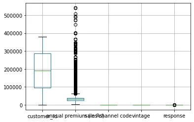
df_final=customerPD[~((customerPD<(Q1-1.5*IQR)) | (customerPD>(Q3+1.5*IQR)))]
df_final=customerPD[~((customerPD<(Q1-1.5*IQR)) | (customerPD>(Q3+1.5*IQR)))]
df_final.boxplot()
<AxesSubplot:>
Q1 = customerD.quantile(0.25)

Q3 = customerD.quantile(0.75)

IQR = Q3 - Q1

print(IQR)
customer_id                190553.0
age                            24.0
driving licence present         0.0
region code                    20.0
previously insured              1.0
dtype: float64
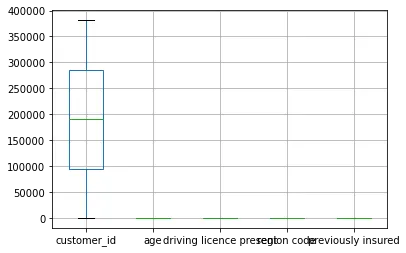
df_final2=customerD[~((customerD<(Q1-1.5*IQR)) | (customerD>(Q3+1.5*IQR)))]
df_final2=customerD[~((customerD<(Q1-1.5*IQR)) | (customerD>(Q3+1.5*IQR)))]
df_final2.boxplot()
<AxesSubplot:>
i. Null values Sum of the null data
customerPD.isnull().sum()
customer_id               387
annual premium (in Rs)    346
sales channel code        400
vintage                   388
response                  361
dtype: int64
customerD.isnull().sum()
customer_id                386
Gender                     368
age                        368
driving licence present    393
region code                392
previously insured         381
vehicle age                381
vehicle damage             407
dtype: int64
Drop Null values for customer_id
customerD["customer_id"].isna().sum()
386
customerPD["customer_id"].isna().sum()
387
customerPD["customer_id"].count()
380722
customerPD["customer_id"].count()
380722
customer_id Drop Null values for customer_id
customerPD=customerPD.dropna(subset=['customer_id'])
Replace all null values for numeric columns by mean
customerPD['annual premium (in Rs)'].fillna((customerPD['annual premium (in Rs)'].mean()), inplace=True)
customerPD['annual premium (in Rs)'].mean()
30563.99977390893
customerPD['vintage'].fillna((customerPD['vintage'].mean()), inplace=True)
customerPD['vintage'].mean()
154.34719220474696
customerPD.isnull().sum()
customer_id                 0
annual premium (in Rs)      0
sales channel code        400
vintage                     0
response                  361
dtype: int64
customerPD['response'].fillna((customerPD['response'].mode()[0]), inplace=True)
customerPD['response'].mode()
0    0.0
dtype: float64
customerPD['sales channel code'].fillna((customerPD['sales channel code'].mode()[0]), inplace=True)
customerPD['sales channel code'].mode()
0    152.0
dtype: float64
___
customerD.isnull().sum()
customer_id                386
Gender                     368
age                        368
driving licence present    393
region code                392
previously insured         381
vehicle age                381
vehicle damage             407
dtype: int64
customer_id Drop Null values for customer_id
customerD=customerD.dropna(subset=['customer_id'])
customerD=customerD.dropna(subset=['vehicle damage'])
customerD=customerD.dropna(subset=['vehicle age'])
customerD=customerD.dropna(subset=['previously insured'])
customerD=customerD.dropna(subset=['region code'])
customerD=customerD.dropna(subset=['driving licence present'])
customerD=customerD.dropna(subset=['Gender'])
customerD.head(2)
| customer_id | Gender | age | driving licence present | region code | previously insured | vehicle age | vehicle damage | |
|---|---|---|---|---|---|---|---|---|
| 0 | 1.0 | Male | 44.0 | 1.0 | 28.0 | 0.0 | > 2 Years | Yes |
| 1 | 2.0 | Male | 76.0 | 1.0 | 3.0 | 0.0 | 1-2 Year | No |
customerD['age'].fillna((customerD['age'].mean()), inplace=True)
#customerD['vehicle age'].fillna((customerD['vehicle age'].mean()), inplace=True)
Feature Engineering
# Unique values for all the columns
for col in customerD.columns[~(customerD.columns.isin(['customer_id']))].tolist():
    print(" Unique Values --> " + col, ':', len(customerD[col].unique()), ': ', customerD[col].unique())
Unique Values --> Gender : 2 :  ['Male' 'Female']
 Unique Values --> age : 67 :  [44.         76.         47.         21.         29.         24.
 23.         56.         32.         41.         71.         37.
 25.         42.         60.         65.         49.         34.
 51.         26.         57.         79.         48.         45.
 72.         30.         54.         27.         38.         22.
 78.         20.         39.         62.         58.         59.
 63.         50.         67.         77.         28.         69.
 52.         31.         33.         43.         36.         53.
 70.         46.         55.         40.         61.         75.
 64.         35.         66.         68.         74.         73.
 84.         83.         81.         38.82120836 80.         82.
 85.        ]
 Unique Values --> driving licence present : 2 :  [1. 0.]
 Unique Values --> region code : 53 :  [28.  3. 11. 41. 33.  6. 35. 50. 15. 45.  8. 36. 30. 26. 16. 47. 48. 19.
 39. 23. 37.  5. 17.  2.  7. 29. 46. 27. 25. 13. 18. 20. 49. 22.  0.  9.
 31. 12. 34. 21. 10. 14. 38. 24. 40. 43. 32. 44.  4. 51. 42.  1. 52.]
 Unique Values --> previously insured : 2 :  [0. 1.]
 Unique Values --> vehicle age : 3 :  ['> 2 Years' '1-2 Year' '< 1 Year']
 Unique Values --> vehicle damage : 2 :  ['Yes' 'No']
customerD=customerD.rename(columns={'driving licence present':'driving_licence_present','previously insured':'previously_insured', 'vehicle age':'vehicle_age', 'vehicle damage':'vehicle_damage'})
Gender = {'Male': 0, 'Female': 1}
#driving_license_present = {0: 0, 1: 1}
previously_insured = {0: 1, 1: 0}
vehicle_age = {'> 2 Years': 2, '1-2 Year': 1, '< 1 Year': 0}
vehicle_damage = {'Yes': 1, 'No': 0}

customerD['Gender'] = customerD['Gender'].map(Gender)
#customerD['driving_license_present'] = customerD['driving_license_present'].map(driving_license_present)
customerD['previously_insured'] = customerD['previously_insured'].map(previously_insured)
customerD['vehicle_age'] = customerD['vehicle_age'].map(vehicle_age)
customerD['vehicle_damage'] = customerD['vehicle_damage'].map(vehicle_damage)
customerD.head(2)
ii. Outliers
(Hint1: for outlier treatment use IQR method as follows:
For example: for a column X calculate Q1 = 25th percentile and Q3 = 75th percentile then IQR = Q3 – Q1 ) then to check outlier, anything lower than a Q1 – 1.5IQR or greater than Q3 + 1.5 IQR would be an outlier
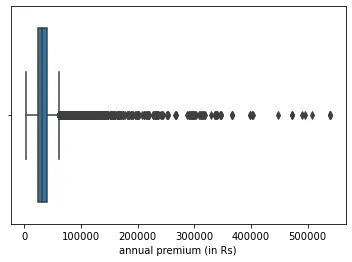
sns.boxplot(customerPD['annual premium (in Rs)'])
<AxesSubplot:xlabel='annual premium (in Rs)'>
percentile25 = customerPD['annual premium (in Rs)'].quantile(0.25)
percentile75 = customerPD['annual premium (in Rs)'].quantile(0.75)
#iqr = np.subtract(*np.percentile(x, [75, 25]))
upper_limit = percentile75 + 1.5 * iqr
lower_limit = percentile25 - 1.5 * iqr
customerPD[customerPD['annual premium (in Rs)'] > upper_limit]
customerPD[customerPD['annual premium (in Rs)'] < lower_limit]
| customer_id | annual premium (in Rs) | sales channel code | vintage | response | |
|---|---|---|---|---|---|
| 5 | 6.0 | 2630.0 | 160.0 | 176.0 | 0.0 |
| 6 | 7.0 | 23367.0 | 152.0 | 249.0 | 0.0 |
| 15 | 16.0 | 2630.0 | 156.0 | 147.0 | 1.0 |
| 27 | 28.0 | 19135.0 | 152.0 | 57.0 | 0.0 |
| 30 | 31.0 | 2630.0 | 160.0 | 136.0 | 0.0 |
| ... | ... | ... | ... | ... | ... |
| 381074 | 381075.0 | 21113.0 | 152.0 | 248.0 | 0.0 |
| 381086 | 381087.0 | 2630.0 | 152.0 | 208.0 | 0.0 |
| 381092 | 381093.0 | 2630.0 | 124.0 | 130.0 | 0.0 |
| 381094 | 381095.0 | 2630.0 | 26.0 | 84.0 | 0.0 |
| 381102 | 381103.0 | 2630.0 | 152.0 | 102.0 | 0.0 |
95172 rows × 5 columns
new_df = customerPD[customerPD['annual premium (in Rs)'] < upper_limit]
new_df.shape
plt.figure(figsize=(16,8))
plt.subplot(2,2,1)
sns.distplot(customerPD['annual premium (in Rs)'])
plt.subplot(2,2,2)
sns.boxplot(customerPD['annual premium (in Rs)'])
plt.subplot(2,2,3)
sns.distplot(new_df['annual premium (in Rs)'])
plt.subplot(2,2,4)
sns.boxplot(new_df['annual premium (in Rs)'])
plt.show()

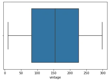
sns.boxplot(customerPD['vintage'])
<AxesSubplot:xlabel='vintage'>
sns.boxplot(customerPD['sales channel code'])
<AxesSubplot:xlabel='sales channel code'>

Outliers customerD
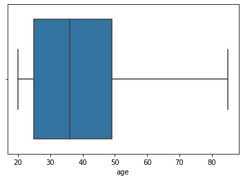
sns.boxplot(customerD['age'])
<AxesSubplot:xlabel='age'>
sns.boxplot(customerD['vehicle_damage'])
<AxesSubplot:xlabel='vehicle_damage'>

sns.boxplot(customerD['previously_insured'])
<AxesSubplot:xlabel='previously_insured'>

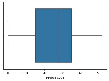
sns.boxplot(customerD['region code'])
<AxesSubplot:xlabel='region code'>
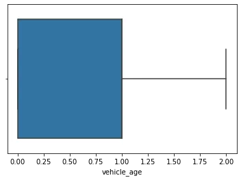
sns.boxplot(customerD['vehicle_age'])
<AxesSubplot:xlabel='vehicle_age'>
Create a Master table for future use. Join the customer table and customer_policy table to get a master table using customer_id in both tables.
(Hint: use pd.merge() function)
customerD['type'] = 'customerD'
customerPD['type'] = 'customerPD'

master_data = pd.concat([customerD, customerPD])
master_data.head(2)
| customer_id | Gender | age | driving_licence_present | region code | previously_insured | vehicle_age | vehicle_damage | type | annual premium (in Rs) | sales channel code | vintage | response | |
|---|---|---|---|---|---|---|---|---|---|---|---|---|---|
| 0 | 1.0 | 0.0 | 44.0 | 1.0 | 28.0 | 1.0 | 2.0 | 1.0 | customerD | NaN | NaN | NaN | NaN |
| 1 | 2.0 | 0.0 | 76.0 | 1.0 | 3.0 | 1.0 | 1.0 | 0.0 | customerD | NaN | NaN | NaN | NaN |
4.Company needs some important information from the master table to make decisions for future growth.They needs following information:
i. Gender wise average annual premium
ii. Age wise average annual premium
iii. Is your data balanced between the genders?
(Hint: Data is balanced if number of counts in each group is approximately same)
iv. Vehicle age wise average annual premium.
plt.figure(figsize = (15, 6))
sns.distplot(master_data.loc[(master_data['Gender'] == 1), 'annual premium (in Rs)'], kde_kws = {"color": "b", "lw": 1, "label": "Male"})
sns.distplot(master_data.loc[(master_data['Gender'] == 0), 'annual premium (in Rs)'], kde_kws = {"color": "r", "lw": 1, "label": "Female"})
plt.title('Age distribution by Gender', fontsize = 15)
plt.show()

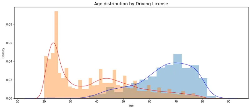
plt.figure(figsize = (15, 6))
sns.distplot(master_data.loc[(master_data['driving_license'] == 0), 'age'], kde_kws = {"color": "b", "lw": 1, "label": "Not Licensed for driving"})
sns.distplot(master_data.loc[(master_data['driving_license'] == 1), 'age'], kde_kws = {"color": "r", "lw": 1, "label": "Licensed for Driving"})
plt.title('Age distribution by Driving License', fontsize = 15)
plt.show()
5
Is there any relation between Person Age and annual premium?
Hint: use correlation function (Correlation describes the relationship between two variables).
Correlation coefficient < -0.5 - Strong negative relationship
Correlation coefficient > 0.5 - Strong positive relationship
0.5 < Correlation coefficient < 0.5 - There is no relationship.
corrMatrix = master_data.corr()
sns.heatmap(corrMatrix, annot = True)
plt.show()