Challenge

Project 2 - EDA on Vehicle Insurance Customer Data

SSurfraz Sharafuddeen13 Jul 2023

Project 2 - EDA on Vehicle Insurance Customer Data

Q 1 Add the column names to both datasets

In [1]:

import pandas as pd

import numpy as np

import seaborn as sns

import matplotlib.pyplot as plt

In [2]:

df1= pd.read_csv('customer_details.csv')

df1

Out[2]:

	0	1	2	3	4	5	6	7
0	1.0	Male	44.0	1.0	28.0	0.0	> 2 Years	Yes
1	2.0	Male	76.0	1.0	3.0	0.0	1-2 Year	No
2	3.0	Male	47.0	1.0	28.0	0.0	> 2 Years	Yes
3	4.0	Male	21.0	1.0	11.0	1.0	< 1 Year	No
4	5.0	Female	29.0	1.0	41.0	1.0	< 1 Year	No
...	...	...	...	...	...	...	...	...
381104	381105.0	Male	74.0	1.0	26.0	1.0	1-2 Year	No
381105	381106.0	Male	30.0	1.0	37.0	1.0	< 1 Year	No
381106	381107.0	Male	21.0	1.0	30.0	1.0	< 1 Year	No
381107	381108.0	Female	68.0	1.0	14.0	0.0	> 2 Years	Yes
381108	381109.0	Male	46.0	1.0	29.0	0.0	1-2 Year	No

381109 rows × 8 columns

In [3]:

df2 = pd.read_csv('customer_policy_details.csv')

df2

Out[3]:

	0	1	2	3	4
0	1.0	40454.0	26.0	217.0	1.0
1	2.0	33536.0	26.0	183.0	0.0
2	3.0	38294.0	26.0	27.0	1.0
3	4.0	28619.0	152.0	203.0	0.0
4	5.0	27496.0	152.0	39.0	0.0
...	...	...	...	...	...
381104	381105.0	30170.0	26.0	88.0	0.0
381105	381106.0	40016.0	152.0	131.0	0.0
381106	381107.0	35118.0	160.0	161.0	0.0
381107	381108.0	44617.0	124.0	74.0	0.0
381108	381109.0	41777.0	26.0	237.0	0.0

381109 rows × 5 columns

Q1 i Column Name for customer details table:

In [4]:

df1.columns = ['customer_id','Gender','age','driving licence present','region code','previously insured','vehicle age','vehicle damage']

df1.head()

Out[4]:

	customer_id	Gender	age	driving licence present	region code	previously insured	vehicle age	vehicle damage
0	1.0	Male	44.0	1.0	28.0	0.0	> 2 Years	Yes
1	2.0	Male	76.0	1.0	3.0	0.0	1-2 Year	No
2	3.0	Male	47.0	1.0	28.0	0.0	> 2 Years	Yes
3	4.0	Male	21.0	1.0	11.0	1.0	< 1 Year	No
4	5.0	Female	29.0	1.0	41.0	1.0	< 1 Year	No

Q1 ii Column Name for customer_policy table:

In [5]:

df2.columns = ['customer_id','annual premium (in Rs)','sales channel code','vintage','response']

df2.head()

Out[5]:

	customer_id	annual premium (in Rs)	sales channel code	vintage	response
0	1.0	40454.0	26.0	217.0	1.0
1	2.0	33536.0	26.0	183.0	0.0
2	3.0	38294.0	26.0	27.0	1.0
3	4.0	28619.0	152.0	203.0	0.0
4	5.0	27496.0	152.0	39.0	0.0

Q2 Checking and Cleaning Data Quality:

i. Null values

df1 null values

In [6]:

df1.isnull().sum()

Out[6]:

customer_id                386
Gender                     368
age                        368
driving licence present    393
region code                392
previously insured         381
vehicle age                381
vehicle damage             407
dtype: int64

In [7]:

df1.dropna(subset=['customer_id'],axis=0,inplace=True)

In [8]:

df1.isnull().sum()

Out[8]:

customer_id                  0
Gender                     368
age                        366
driving licence present    392
region code                391
previously insured         381
vehicle age                381
vehicle damage             406
dtype: int64

In [9]:

df1['age'].fillna(df1['age'].mean(),inplace=True)

In [10]:

df1.isnull().sum()

Out[10]:

customer_id                  0
Gender                     368
age                          0
driving licence present    392
region code                391
previously insured         381
vehicle age                381
vehicle damage             406
dtype: int64

In [11]:

df1['Gender'].fillna(df1['Gender'].mode()[0],inplace=True)

df1['driving licence present'].fillna(df1['driving licence present'].mode()[0],inplace=True)

df1['region code'].fillna(df1['region code'].mode()[0],inplace=True)

df1['previously insured'].fillna(df1['previously insured'].mode()[0],inplace=True)

df1['vehicle age'].fillna(df1['vehicle age'].mode()[0],inplace=True)

df1['vehicle damage'].fillna(df1['vehicle damage'].mode()[0],inplace=True)

In [12]:

df1.isnull().sum()

Out[12]:

customer_id                0
Gender                     0
age                        0
driving licence present    0
region code                0
previously insured         0
vehicle age                0
vehicle damage             0
dtype: int64

In [13]:

df1

Out[13]:

	customer_id	Gender	age	driving licence present	region code	previously insured	vehicle age	vehicle damage
0	1.0	Male	44.0	1.0	28.0	0.0	> 2 Years	Yes
1	2.0	Male	76.0	1.0	3.0	0.0	1-2 Year	No
2	3.0	Male	47.0	1.0	28.0	0.0	> 2 Years	Yes
3	4.0	Male	21.0	1.0	11.0	1.0	< 1 Year	No
4	5.0	Female	29.0	1.0	41.0	1.0	< 1 Year	No
...	...	...	...	...	...	...	...	...
381104	381105.0	Male	74.0	1.0	26.0	1.0	1-2 Year	No
381105	381106.0	Male	30.0	1.0	37.0	1.0	< 1 Year	No
381106	381107.0	Male	21.0	1.0	30.0	1.0	< 1 Year	No
381107	381108.0	Female	68.0	1.0	14.0	0.0	> 2 Years	Yes
381108	381109.0	Male	46.0	1.0	29.0	0.0	1-2 Year	No

380723 rows × 8 columns

df2 null values

In [14]:

df2.isnull().sum()

Out[14]:

customer_id               387
annual premium (in Rs)    346
sales channel code        400
vintage                   388
response                  361
dtype: int64

In [15]:

df2.dropna(subset=['customer_id'],axis=0,inplace=True)

In [16]:

df2.isnull().sum()

Out[16]:

customer_id                 0
annual premium (in Rs)    344
sales channel code        400
vintage                   388
response                  361
dtype: int64

In [17]:

df2.head()

Out[17]:

	customer_id	annual premium (in Rs)	sales channel code	vintage	response
0	1.0	40454.0	26.0	217.0	1.0
1	2.0	33536.0	26.0	183.0	0.0
2	3.0	38294.0	26.0	27.0	1.0
3	4.0	28619.0	152.0	203.0	0.0
4	5.0	27496.0	152.0	39.0	0.0

In [18]:

df2['annual premium (in Rs)'].fillna(df2['annual premium (in Rs)'].mean(),inplace=True)

In [19]:

df2.isnull().sum()

Out[19]:

customer_id                 0
annual premium (in Rs)      0
sales channel code        400
vintage                   388
response                  361
dtype: int64

In [20]:

df2['vintage'].fillna(df2['vintage'].mean(),inplace=True)

In [21]:

df2.isnull().sum()

Out[21]:

customer_id                 0
annual premium (in Rs)      0
sales channel code        400
vintage                     0
response                  361
dtype: int64

In [22]:

df2['sales channel code'].fillna(df2['sales channel code'].mode()[0],inplace=True)

df2['response'].fillna(df2['response'].mode()[0],inplace=True

In [23]:

df2.isnull().sum()

Out[23]:

customer_id               0
annual premium (in Rs)    0
sales channel code        0
vintage                   0
response                  0
dtype: int64

In [24]:

df2

Out[24]:

	customer_id	annual premium (in Rs)	sales channel code	vintage	response
0	1.0	40454.0	26.0	217.0	1.0
1	2.0	33536.0	26.0	183.0	0.0
2	3.0	38294.0	26.0	27.0	1.0
3	4.0	28619.0	152.0	203.0	0.0
4	5.0	27496.0	152.0	39.0	0.0
...	...	...	...	...	...
381104	381105.0	30170.0	26.0	88.0	0.0
381105	381106.0	40016.0	152.0	131.0	0.0
381106	381107.0	35118.0	160.0	161.0	0.0
381107	381108.0	44617.0	124.0	74.0	0.0
381108	381109.0	41777.0	26.0	237.0	0.0

380722 rows × 5 columns

Q2 ii Outliers

df1 outliers

In [25]:

df1.describe()

Out[25]:

	customer_id	age	driving licence present	region code	previously insured
count	380723.000000	380723.000000	380723.000000	380723.000000	380723.000000
mean	190548.776244	38.822788	0.997870	26.391090	0.457800
std	110016.805160	15.504826	0.046105	13.223772	0.498217
min	1.000000	20.000000	0.000000	0.000000	0.000000
25%	95269.500000	25.000000	1.000000	15.000000	0.000000
50%	190543.000000	36.000000	1.000000	28.000000	0.000000
75%	285822.500000	49.000000	1.000000	35.000000	1.000000
max	381109.000000	85.000000	1.000000	52.000000	1.000000

In [26]:

df1_q1 = df1.quantile(0.25)

df1_q3 = df1.quantile(0.75)

df1_IQR = df1_q3 - df1_q1

In [27]:

df1_lower = df1_q1 - 1.5 * df1_IQR

df1_lower

Out[27]:

customer_id               -190560.0
age                           -11.0
driving licence present         1.0
region code                   -15.0
previously insured             -1.5
dtype: float64

In [28]:

df1_upper = df1_q3 + 1.5 * df1_IQR

df1_upper

Out[28]:

customer_id                571652.0
age                            85.0
driving licence present         1.0
region code                    65.0
previously insured              2.5
dtype: float64

In [29]:

((df1 < df1_lower) | (df1 > df1_upper)).sum()

Out[29]:

Gender                       0
age                          0
customer_id                  0
driving licence present    811
previously insured           0
region code                  0
vehicle age                  0
vehicle damage               0
dtype: int64

In [30]:

# Only column 'driving licence present' present in outlier,

In [31]:

def replace_outliers(df):

    q1=df.quantile(0.25)

    q3=df.quantile(0.75)

    IQR=q3-q1

    upper = df[~(df>(q3+1.5*IQR))].max()

    lower = df[~(df<(q1-1.5*IQR))].min()

    df = np.where(df > upper, df.mean(),np.where(df < lower,df.mean(),df))

    return df

In [32]:

replace_outliers(df1['driving licence present'])

Out[32]:

array([1., 1., 1., ..., 1., 1., 1.])

In [33]:

df1.describe()

Out[33]:

	customer_id	age	driving licence present	region code	previously insured
count	380723.000000	380723.000000	380723.000000	380723.000000	380723.000000
mean	190548.776244	38.822788	0.997870	26.391090	0.457800
std	110016.805160	15.504826	0.046105	13.223772	0.498217
min	1.000000	20.000000	0.000000	0.000000	0.000000
25%	95269.500000	25.000000	1.000000	15.000000	0.000000
50%	190543.000000	36.000000	1.000000	28.000000	0.000000
75%	285822.500000	49.000000	1.000000	35.000000	1.000000
max	381109.000000	85.000000	1.000000	52.000000	1.000000

df2 outliers

In [34]:

df2.describe()

Out[34]:

	customer_id	annual premium (in Rs)	sales channel code	vintage	response
count	380722.000000	380722.000000	380722.000000	380722.000000	380722.000000
mean	190547.491663	30563.999774	112.078674	154.347192	0.122410
std	110013.824148	17190.147550	54.192513	83.628096	0.327759
min	1.000000	2630.000000	1.000000	10.000000	0.000000
25%	95276.250000	24416.000000	29.000000	82.000000	0.000000
50%	190536.500000	31656.000000	136.000000	154.000000	0.000000
75%	285818.750000	39391.750000	152.000000	227.000000	0.000000
max	381109.000000	540165.000000	163.000000	299.000000	1.000000

In [35]:

df2_q1 = df2.quantile(0.25)

df2_q3 = df2.quantile(0.75)

df2_IQR = df2_q3 - df2_q1

In [36]:

df2_lower = df2_q1 - 1.5 * df2_IQR

df2_lower

Out[36]:

customer_id              -190537.500
annual premium (in Rs)      1952.375
sales channel code          -155.500
vintage                     -135.500
response                       0.000
dtype: float64

In [37]:

df2_upper = df2_q3 + 1.5 * df2_IQR

df2_upper

Out[37]:

customer_id               571632.500
annual premium (in Rs)     61855.375
sales channel code           336.500
vintage                      444.500
response                       0.000
dtype: float64

In [38]:

((df2 < df2_lower) | (df2 > df2_upper)).sum()

Out[38]:

customer_id                   0
annual premium (in Rs)    10332
sales channel code            0
vintage                       0
response                  46604
dtype: int64

In [39]:

# In df2, columns 'annual premium (in Rs)' & 'response' are showing as outliers, of which only 'annual premium (in Rs)' column

# is numeric and 'response' column is categorical. Hence, only mean of 'annual premium (in Rs)' column is calculated.

In [40]:

replace_outliers(df2['annual premium (in Rs)'])

replace_outliers(df2['response'])

Out[40]:

array([0.12240953, 0.        , 0.12240953, ..., 0.        , 0.        ,
       0.        ])

In [41]:

df2.describe()

Out[41]:

	customer_id	annual premium (in Rs)	sales channel code	vintage	response
count	380722.000000	380722.000000	380722.000000	380722.000000	380722.000000
mean	190547.491663	30563.999774	112.078674	154.347192	0.122410
std	110013.824148	17190.147550	54.192513	83.628096	0.327759
min	1.000000	2630.000000	1.000000	10.000000	0.000000
25%	95276.250000	24416.000000	29.000000	82.000000	0.000000
50%	190536.500000	31656.000000	136.000000	154.000000	0.000000
75%	285818.750000	39391.750000	152.000000	227.000000	0.000000
max	381109.000000	540165.000000	163.000000	299.000000	1.000000

Q2 iii. White spaces

In [42]:

df1.head()

Out[42]:

	customer_id	Gender	age	driving licence present	region code	previously insured	vehicle age	vehicle damage
0	1.0	Male	44.0	1.0	28.0	0.0	> 2 Years	Yes
1	2.0	Male	76.0	1.0	3.0	0.0	1-2 Year	No
2	3.0	Male	47.0	1.0	28.0	0.0	> 2 Years	Yes
3	4.0	Male	21.0	1.0	11.0	1.0	< 1 Year	No
4	5.0	Female	29.0	1.0	41.0	1.0	< 1 Year	No

In [43]:

df1['Gender'] = df1['Gender'].str.strip()

df1['vehicle age'] = df1['vehicle age'].str.strip()

df1['vehicle damage'] = df1['vehicle damage'].str.strip()

In [44]:

df2.head()

Out[44]:

	customer_id	annual premium (in Rs)	sales channel code	vintage	response
0	1.0	40454.0	26.0	217.0	1.0
1	2.0	33536.0	26.0	183.0	0.0
2	3.0	38294.0	26.0	27.0	1.0
3	4.0	28619.0	152.0	203.0	0.0
4	5.0	27496.0	152.0	39.0	0.0

In [45]:

# As df2 contains only numerical values and white spaces can only be detected in string value.

Q 2 iv. case correction(lower or upper, any one)

In [46]:

df1.head()

Out[46]:

	customer_id	Gender	age	driving licence present	region code	previously insured	vehicle age	vehicle damage
0	1.0	Male	44.0	1.0	28.0	0.0	> 2 Years	Yes
1	2.0	Male	76.0	1.0	3.0	0.0	1-2 Year	No
2	3.0	Male	47.0	1.0	28.0	0.0	> 2 Years	Yes
3	4.0	Male	21.0	1.0	11.0	1.0	< 1 Year	No
4	5.0	Female	29.0	1.0	41.0	1.0	< 1 Year	No

In [47]:

df1['Gender'] = df1['Gender'].str.upper()

df1['vehicle age'] = df1['vehicle age'].str.upper()

df1['vehicle damage'] = df1['vehicle damage'].str.upper()

In [48]:

df1.head()

Out[48]:

	customer_id	Gender	age	driving licence present	region code	previously insured	vehicle age	vehicle damage
0	1.0	MALE	44.0	1.0	28.0	0.0	> 2 YEARS	YES
1	2.0	MALE	76.0	1.0	3.0	0.0	1-2 YEAR	NO
2	3.0	MALE	47.0	1.0	28.0	0.0	> 2 YEARS	YES
3	4.0	MALE	21.0	1.0	11.0	1.0	< 1 YEAR	NO
4	5.0	FEMALE	29.0	1.0	41.0	1.0	< 1 YEAR	NO

In [49]:

# df1 is the dataframe that contains string values. df2 contains only numerical values

Q2 v. Convert nominal data (categorical) into dummies

df1

In [50]:

Gender_dummy = pd.get_dummies(df1['Gender'])

Gender_dummy

Out[50]:

	FEMALE	MALE
0	0	1
1	0	1
2	0	1
3	0	1
4	1	0
...	...	...
381104	0	1
381105	0	1
381106	0	1
381107	1	0
381108	0	1

380723 rows × 2 columns

In [51]:

Drivinglicense_dummy = pd.get_dummies(df1['driving licence present'])

Drivinglicense_dummy

Out[51]:

	0.0	1.0
0	0	1
1	0	1
2	0	1
3	0	1
4	0	1
...	...	...
381104	0	1
381105	0	1
381106	0	1
381107	0	1
381108	0	1

380723 rows × 2 columns

In [52]:

region_dummy = pd.get_dummies(df1['region code'])

region_dummy

Out[52]:

	0.0	1.0	2.0	3.0	4.0	5.0	6.0	7.0	8.0	9.0	...	43.0	44.0	45.0	46.0	47.0	48.0	49.0	50.0	51.0	52.0
0	0	0	0	0	0	0	0	0	0	0	...	0	0	0	0	0	0	0	0	0	0
1	0	0	0	1	0	0	0	0	0	0	...	0	0	0	0	0	0	0	0	0	0
2	0	0	0	0	0	0	0	0	0	0	...	0	0	0	0	0	0	0	0	0	0
3	0	0	0	0	0	0	0	0	0	0	...	0	0	0	0	0	0	0	0	0	0
4	0	0	0	0	0	0	0	0	0	0	...	0	0	0	0	0	0	0	0	0	0
...	...	...	...	...	...	...	...	...	...	...	...	...	...	...	...	...	...	...	...	...	...
381104	0	0	0	0	0	0	0	0	0	0	...	0	0	0	0	0	0	0	0	0	0
381105	0	0	0	0	0	0	0	0	0	0	...	0	0	0	0	0	0	0	0	0	0
381106	0	0	0	0	0	0	0	0	0	0	...	0	0	0	0	0	0	0	0	0	0
381107	0	0	0	0	0	0	0	0	0	0	...	0	0	0	0	0	0	0	0	0	0
381108	0	0	0	0	0	0	0	0	0	0	...	0	0	0	0	0	0	0	0	0	0

380723 rows × 53 columns

In [53]:

previousins_dummy = pd.get_dummies(df1['previously insured'])

previousins_dummy

Out[53]:

	0.0	1.0
0	1	0
1	1	0
2	1	0
3	0	1
4	0	1
...	...	...
381104	0	1
381105	0	1
381106	0	1
381107	1	0
381108	1	0

380723 rows × 2 columns

In [54]:

vehicleage_dummy = pd.get_dummies(df1['vehicle age'])

vehicleage_dummy

Out[54]:

	1-2 YEAR	< 1 YEAR	> 2 YEARS
0	0	0	1
1	1	0	0
2	0	0	1
3	0	1	0
4	0	1	0
...	...	...	...
381104	1	0	0
381105	0	1	0
381106	0	1	0
381107	0	0	1
381108	1	0	0

380723 rows × 3 columns

In [55]:

vehicledamage_dummy = pd.get_dummies(df1['vehicle damage'])

vehicledamage_dummy

Out[55]:

	NO	YES
0	0	1
1	1	0
2	0	1
3	1	0
4	1	0
...	...	...
381104	1	0
381105	1	0
381106	1	0
381107	0	1
381108	1	0

380723 rows × 2 columns

df2

In [56]:

df2.head()

Out[56]:

	customer_id	annual premium (in Rs)	sales channel code	vintage	response
0	1.0	40454.0	26.0	217.0	1.0
1	2.0	33536.0	26.0	183.0	0.0
2	3.0	38294.0	26.0	27.0	1.0
3	4.0	28619.0	152.0	203.0	0.0
4	5.0	27496.0	152.0	39.0	0.0

In [57]:

saleschannel_dummy = pd.get_dummies(df2['sales channel code'])

saleschannel_dummy

Out[57]:

	1.0	2.0	3.0	4.0	6.0	7.0	8.0	9.0	10.0	11.0	...	152.0	153.0	154.0	155.0	156.0	157.0	158.0	159.0	160.0	163.0
0	0	0	0	0	0	0	0	0	0	0	...	0	0	0	0	0	0	0	0	0	0
1	0	0	0	0	0	0	0	0	0	0	...	0	0	0	0	0	0	0	0	0	0
2	0	0	0	0	0	0	0	0	0	0	...	0	0	0	0	0	0	0	0	0	0
3	0	0	0	0	0	0	0	0	0	0	...	1	0	0	0	0	0	0	0	0	0
4	0	0	0	0	0	0	0	0	0	0	...	1	0	0	0	0	0	0	0	0	0
...	...	...	...	...	...	...	...	...	...	...	...	...	...	...	...	...	...	...	...	...	...
381104	0	0	0	0	0	0	0	0	0	0	...	0	0	0	0	0	0	0	0	0	0
381105	0	0	0	0	0	0	0	0	0	0	...	1	0	0	0	0	0	0	0	0	0
381106	0	0	0	0	0	0	0	0	0	0	...	0	0	0	0	0	0	0	0	1	0
381107	0	0	0	0	0	0	0	0	0	0	...	0	0	0	0	0	0	0	0	0	0
381108	0	0	0	0	0	0	0	0	0	0	...	0	0	0	0	0	0	0	0	0	0

380722 rows × 155 columns

In [58]:

response_dummy = pd.get_dummies(df2['response'])

response_dummy

Out[58]:

	0.0	1.0
0	0	1
1	1	0
2	0	1
3	1	0
4	1	0
...	...	...
381104	1	0
381105	1	0
381106	1	0
381107	1	0
381108	1	0

380722 rows × 2 columns

Q2 vi. Drop Duplicates (duplicated rows)

In [59]:

df1 = df1.drop_duplicates()

df1

Out[59]:

	customer_id	Gender	age	driving licence present	region code	previously insured	vehicle age	vehicle damage
0	1.0	MALE	44.0	1.0	28.0	0.0	> 2 YEARS	YES
1	2.0	MALE	76.0	1.0	3.0	0.0	1-2 YEAR	NO
2	3.0	MALE	47.0	1.0	28.0	0.0	> 2 YEARS	YES
3	4.0	MALE	21.0	1.0	11.0	1.0	< 1 YEAR	NO
4	5.0	FEMALE	29.0	1.0	41.0	1.0	< 1 YEAR	NO
...	...	...	...	...	...	...	...	...
381104	381105.0	MALE	74.0	1.0	26.0	1.0	1-2 YEAR	NO
381105	381106.0	MALE	30.0	1.0	37.0	1.0	< 1 YEAR	NO
381106	381107.0	MALE	21.0	1.0	30.0	1.0	< 1 YEAR	NO
381107	381108.0	FEMALE	68.0	1.0	14.0	0.0	> 2 YEARS	YES
381108	381109.0	MALE	46.0	1.0	29.0	0.0	1-2 YEAR	NO

380723 rows × 8 columns

In [60]:

df2 = df2.drop_duplicates()

df2

Out[60]:

	customer_id	annual premium (in Rs)	sales channel code	vintage	response
0	1.0	40454.0	26.0	217.0	1.0
1	2.0	33536.0	26.0	183.0	0.0
2	3.0	38294.0	26.0	27.0	1.0
3	4.0	28619.0	152.0	203.0	0.0
4	5.0	27496.0	152.0	39.0	0.0
...	...	...	...	...	...
381104	381105.0	30170.0	26.0	88.0	0.0
381105	381106.0	40016.0	152.0	131.0	0.0
381106	381107.0	35118.0	160.0	161.0	0.0
381107	381108.0	44617.0	124.0	74.0	0.0
381108	381109.0	41777.0	26.0	237.0	0.0

380722 rows × 5 columns

Q3. Create a Master table for future use

In [61]:

master=pd.merge(df1,df2,on='customer_id')

master

Out[61]:

	customer_id	Gender	age	driving licence present	region code	previously insured	vehicle age	vehicle damage	annual premium (in Rs)	sales channel code	vintage	response
0	1.0	MALE	44.0	1.0	28.0	0.0	> 2 YEARS	YES	40454.0	26.0	217.0	1.0
1	2.0	MALE	76.0	1.0	3.0	0.0	1-2 YEAR	NO	33536.0	26.0	183.0	0.0
2	3.0	MALE	47.0	1.0	28.0	0.0	> 2 YEARS	YES	38294.0	26.0	27.0	1.0
3	4.0	MALE	21.0	1.0	11.0	1.0	< 1 YEAR	NO	28619.0	152.0	203.0	0.0
4	5.0	FEMALE	29.0	1.0	41.0	1.0	< 1 YEAR	NO	27496.0	152.0	39.0	0.0
...	...	...	...	...	...	...	...	...	...	...	...	...
380331	381105.0	MALE	74.0	1.0	26.0	1.0	1-2 YEAR	NO	30170.0	26.0	88.0	0.0
380332	381106.0	MALE	30.0	1.0	37.0	1.0	< 1 YEAR	NO	40016.0	152.0	131.0	0.0
380333	381107.0	MALE	21.0	1.0	30.0	1.0	< 1 YEAR	NO	35118.0	160.0	161.0	0.0
380334	381108.0	FEMALE	68.0	1.0	14.0	0.0	> 2 YEARS	YES	44617.0	124.0	74.0	0.0
380335	381109.0	MALE	46.0	1.0	29.0	0.0	1-2 YEAR	NO	41777.0	26.0	237.0	0.0

380336 rows × 12 columns

Q 4 i. Gender wise average annual premium

In [62]:

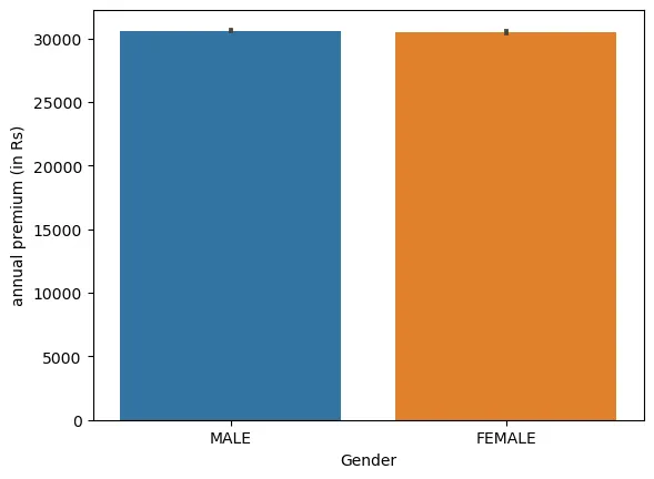
gender_premium = master.groupby('Gender')['annual premium (in Rs)']

gender_premium.mean()

Out[62]:

Gender
FEMALE    30492.028478
MALE      30623.619273
Name: annual premium (in Rs), dtype: float64

In [63]:

sns.barplot(data=master,x='Gender',y='annual premium (in Rs)')

plt.show()

In [64]:

# It can be noted that the annual premium is similar for both genders and is not gender biased.

Q 4 ii. Age wise average annual premium

In [65]:

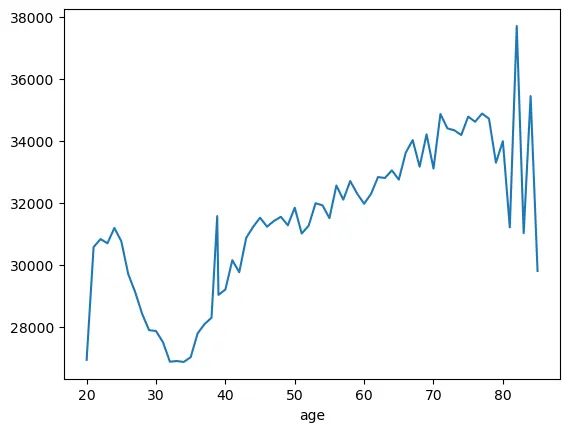
age_premium = master.groupby('age')['annual premium (in Rs)']

age_premium.mean()

Out[65]:

age
20.0    26924.620173
21.0    30564.475810
22.0    30823.778102
23.0    30688.606298
24.0    31183.802890
            ...     
81.0    31201.571429
82.0    37705.379310
83.0    31012.727273
84.0    35440.818182
85.0    29792.363636
Name: annual premium (in Rs), Length: 67, dtype: float64

In [66]:

age_premium.mean().plot()

plt.show()

Q 4 iii. Is your data balanced between the genders?

In [67]:

count_gender = master.groupby(['Gender']).count()

count_gender

Out[67]:

	customer_id	age	driving licence present	region code	previously insured	vehicle age	vehicle damage	annual premium (in Rs)	sales channel code	vintage	response
Gender
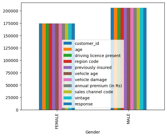
FEMALE	174485	174485	174485	174485	174485	174485	174485	174485	174485	174485	174485
MALE	205851	205851	205851	205851	205851	205851	205851	205851	205851	205851	205851

In [68]:

count_gender.iloc[0]

Out[68]:

customer_id                174485
age                        174485
driving licence present    174485
region code                174485
previously insured         174485
vehicle age                174485
vehicle damage             174485
annual premium (in Rs)     174485
sales channel code         174485
vintage                    174485
response                   174485
Name: FEMALE, dtype: int64

In [69]:

count_gender.iloc[1]

Out[69]:

customer_id                205851
age                        205851
driving licence present    205851
region code                205851
previously insured         205851
vehicle age                205851
vehicle damage             205851
annual premium (in Rs)     205851
sales channel code         205851
vintage                    205851
response                   205851
Name: MALE, dtype: int64

In [86]:

count_gender.plot.bar(xlabel='Gender')

plt.legend(loc=0)

plt.show()

In [71]:

# The above chart proves that the data is balanced between the genders as number of counts in each group is approximately same.

Q 4 iv. Vehicle age wise average annual premium.

In [72]:

master.head()

Out[72]:

	customer_id	Gender	age	driving licence present	region code	previously insured	vehicle age	vehicle damage	annual premium (in Rs)	sales channel code	vintage	response
0	1.0	MALE	44.0	1.0	28.0	0.0	> 2 YEARS	YES	40454.0	26.0	217.0	1.0
1	2.0	MALE	76.0	1.0	3.0	0.0	1-2 YEAR	NO	33536.0	26.0	183.0	0.0
2	3.0	MALE	47.0	1.0	28.0	0.0	> 2 YEARS	YES	38294.0	26.0	27.0	1.0
3	4.0	MALE	21.0	1.0	11.0	1.0	< 1 YEAR	NO	28619.0	152.0	203.0	0.0
4	5.0	FEMALE	29.0	1.0	41.0	1.0	< 1 YEAR	NO	27496.0	152.0	39.0	0.0

In [73]:

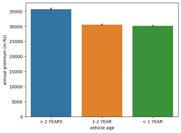
vehicle_age_premium = master.groupby('vehicle age')['annual premium (in Rs)']

vehicle_age_premium.mean()

Out[73]:

vehicle age
1-2 YEAR     30524.629840
< 1 YEAR     30115.716367
> 2 YEARS    35657.520845
Name: annual premium (in Rs), dtype: float64

In [74]:

sns.barplot(x='vehicle age',y='annual premium (in Rs)',data=master)

plt.show()

Q 5. Is there any relation between Person Age and annual premium

In [75]:

Correlation_coefficient = master['age'].corr(master['annual premium (in Rs)'])

Correlation_coefficient

Out[75]:

0.06771515986613913

In [76]:

if Correlation_coefficient < -0.5:

    print('Strong negative relationship')

elif Correlation_coefficient > 0.5:

    print('Strong positive relationship')

elif 0.5 < Correlation_coefficient and Correlation_coefficient < 0.5:

    print('There is no relationship')

else:

    print('There is good relationship')

There is good relationship

In [77]:

master[['age','annual premium (in Rs)']].corr()

Out[77]:

	age	annual premium (in Rs)
age	1.000000	0.067715
annual premium (in Rs)	0.067715	1.000000

In [ ]:

Project 2 - EDA on Vehicle Insurance Customer Data

Project 2 - EDA on Vehicle Insurance Customer Data

Q 1 Add the column names to both datasets

Q1 i Column Name for customer details table:

Q1 ii Column Name for customer_policy table:

Q2 Checking and Cleaning Data Quality:

i. Null values

df1 null values

df2 null values

Q2 ii Outliers

df1 outliers

df2 outliers

Q2 iii. White spaces

Q 2 iv. case correction(lower or upper, any one)

Q2 v. Convert nominal data (categorical) into dummies

df1

Q 4 ii. Age wise average annual premium

Q 4 iii. Is your data balanced between the genders?

Q 4 iv. Vehicle age wise average annual premium.

Q 5. Is there any relation between Person Age and annual premium

Ship work like this
in your own course.

Talk to a career counsellor

Project 2 - EDA on Vehicle Insurance Customer Data

Q 1 Add the column names to both datasets

Q1 i Column Name for customer details table:

Q1 ii Column Name for customer_policy table:

Q2 Checking and Cleaning Data Quality:

i. Null values

df1 null values

df2 null values

Q2 ii Outliers

df1 outliers

df2 outliers

Q2 iii. White spaces

Q 2 iv. case correction(lower or upper, any one)

Q2 v. Convert nominal data (categorical) into dummies

df1

Q 4 ii. Age wise average annual premium

Q 4 iii. Is your data balanced between the genders?

Q 4 iv. Vehicle age wise average annual premium.

Q 5. Is there any relation between Person Age and annual premium

Ship work like thisin your own course.

Talk to a career counsellor

Ship work like this
in your own course.