Project 2

AIM:

• development of a forward energy-based fuel consumption model of a P1 hybrid vehicle.
• quantify the improvement in fuel economy numbers for the hybrid vehicle [kmpl], compared to the conventional vehicle, on the urban cycle [UDDS] and highway cycle [HWFET].
• to analyse and understand the vehicle operating points in terms of engine and motor speed, torque, transmission speeds, pedal positions, gear, distance travelled, battery voltage, current, SoC etc.
• write pre-processing scripts in MATLAB to load all the variable needed to run the Simulink model.
• Modify conventional vehicle Simulink model into a hybrid vehicle model.
• analyse data and write post-processing scripts in MATLAB to create plots using MATLAB scripts.

OBJECTIVES:

1. Tabulate the fuel economy numbers [kmpl] for UDDS and HWFET cycle. Compare these numbers with the baseline numbers for conventional vehicle model.
2. Plot the time trace for engine, transmission input, transmission output and wheel speed on one plot.
3. Plot engine torque, engine power, fuel rate and fuel consumption using subplots.
4. Plot accelerator and brake pedal, gear command, vehicle desired and actual speed, vehicle distance using subplots.
5. Plot the engine operating points on the engine fuel map.
6. Plot motor speed, torque, motor input power using subplots.
7. Plot pack voltage, current and SoC using subplots.
8. Plot the motor operating points on the motor input power map, with the motor max motoring and generating torque curves.
9. Write down appropriate brief comments on each of these plots, describing the vehicle behaviour throughout the drive cycle.
10. Generate the plots for both drive cycles

Forward Model Approach:

• the forward modelling approach is also called as cause-effect, engine to wheel method.
• the direction of calculation is the same as the direction of positive power flow from engine to wheel.
• this approach is based on vehicle dynamics equation and the behaviour of each powertrain components and their dynamics interaction.
• in this we start with modelled using a ‘Driver' block, which is a basic PI controller that generates accelerator and brake pedal outputs to match the desired and actual vehicle speeds.
• The ‘Controller’ block is the brains of the vehicle, representing the electronic controls units. Based on the driver inputs, it generates desired engine torque, desired transmission gear and desired brake torque.
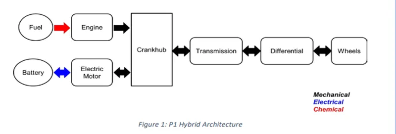
• These inputs are fed to the ‘Powertrain’ block which represents the drivetrain of the vehicle. It consists of an ‘Engine’ and 'Electric Motor through battery' connected to the ‘Automatic Transmission’ through a ‘Torque Converter’. The output of the transmission is connected to the ’Differential’, which powers the ‘Wheels’, that provides the tractive force for vehicle acceleration. The longitudinal dynamics of the vehicle along with the road load is represented in the ‘Vehicle Dynamics’ block.

Honda Insight motor and battery are considered for this project. Data is taken from ADVISOR data base developed by NREL, USA. Data provided in the project files.

MATLAB Code:

%%%%%%%%%%%%%%%%%%%%%%%%%%%%%%%%%%%%%%%%%%%%%%%%%%%%%%%%%%%%%%%%%%%%%

%% Skill-Lync -> Hybrid Drives Development

% Project 1 - Conventional Vehicle Model

% By – Abhishek kumar singh

% Description:

%% Initialization File

% Initialization file for loading the variables for the Conventional vehicle simulation model

close all

clear; clc;

%% Vehicle Parameters

M = 1500; % Vehicle weight [kg]

Cr = 0.015; % Rolling resistance coefficient

Rw = 0.35; % Rolling radius [m]

Cd = 0.33; % Drag coefficient

Af = 2; % Frontal area [m2]

rhoa = 1.225; % Air density [kg/m3]

Vwind = 0; % Wind velocity [kmph]

g = 9.81; % Gravitational acceleration [m/s2]

theta = 0; % Slope [deg]

myu_road_tire = 1; % Coefficient of friction between tire - road interface

%% Powertrain Parameters

FDR = 3.73; % Final Drive Ratio / Diff Ratio

DiffEff = 0.99; % Differential efficiency (assumed independent of operating conditions)

NumGear = 4; % Number of gears in transmission

TransGear = 1:NumGear; % Transmission Gears

TransRatio = [3.06, 1.62, 1, 0.7]; % Corresponding Transmission ratios

TransEff = 0.90; % Transmission efficiency (assumed independent of operating conditions)

TC_SR = [0, .5, .6, .7, .8, .87, .92, .94, .96, .97, 1]; % Torque Converter Speed Ratio (Matlab default) -> TurbSpd/PumpSpd

TC_TR = [2.232, 1.5462, 1.4058, 1.2746, 1.1528, 1.0732, 1.0192, 1, 1, 1, 1]; % Torque Converter Torque Ratio (Matlab default) -> TurbTrq/PumpTrq

TC_Cf = 1e-4 * [.72558, .66322, .63463, .59042, .51331, .4144, .29287, .22444, .12186, .04386, 0]; % Torque Converter Capacity Factor (Matlab default) -> PumpTrq/PumpSpd^2 [Nm/rpm^2]

load Vehicle_Data/Engine_data_1_9L_Saturn_95kW

load Vehicle_Data/Trans_Shift_map

load Vehicle_Data/EM_Honda_Insight_10kW

load Vehicle_Data/ESS_NiMH6

ESS_init_soc = 0.8;

ESS_soc_max = 0.9;

ESS_soc_min = 0.6;

%% Driver Parameters

Kp = 10; % P gain for driver PI model

Ki = 1; % I gain for driver PI model

%% Inputting the desired DriveCycle

Drive_Cycle_Select = input(sprintf('Select a Drive Cycle: \n 1. UDDS \n 2. HWFET \n 3. FTP \n 4. US06 \n 5. NEDC \n 6. WLTP \n Drive_Cycle_Select: '));

% Drive cycle selection

% Drive cycle values in m/s

if Drive_Cycle_Select == 1

load DriveCycles/UDDS;

elseif Drive_Cycle_Select == 2

load DriveCycles/HWFET;

elseif Drive_Cycle_Select == 3

load DriveCycles/FTP;

elseif Drive_Cycle_Select == 4

load DriveCycles/US06;

elseif Drive_Cycle_Select == 5

load DriveCycles/NEDC;

elseif Drive_Cycle_Select == 6

load DriveCycles/WLTP;

end

time_end = cyc_time(end);

vel_end = cyc_vel(end);

This code is designed such a way that it asks for the drive cycle that need to be used for the study and the user input decides the desired drive cycle for the study. The screenshot of the command window asking for the drive cycle of study is shown in figure. For the chosen drive cycle the Simulink vehicle model will be run automatically, and after that MATLAB post processing script will be run automatically for providing the necessary plots for the study.

By running the above script, you will get this in command window:

Select a Drive Cycle:

1. UDDS
2. HWFET
3. FTP
4. US06
5. NEDC
6. WLTP

Drive_Cycle_Select: 1/2/3/4/5/6 whichever is required.

Simulink Model:

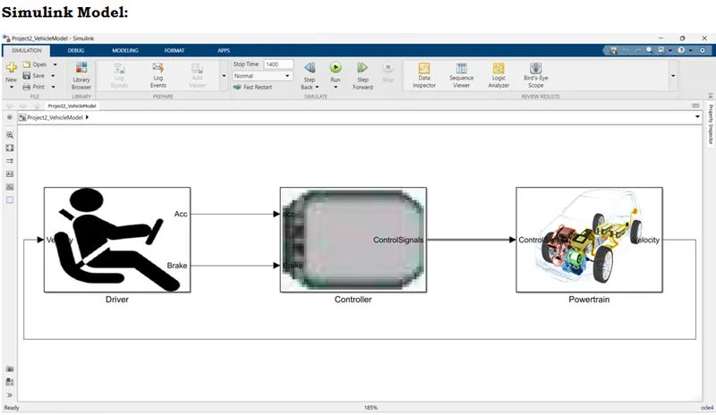
Here we start with modelled using a Driver model block, which is a basic PI controller that generates accelerator and brake pedal outputs to match the desired and actual vehicle speeds.

The Controller model block is the brains of the vehicle, representing the electronic controls units. Based on the driver inputs, it generates desired engine torque, desired transmission gear and desired brake torque.

These inputs are fed to the Powertrain model block which represents the drivetrain of the vehicle. It consists of an Engine model with Electric Motor connected to the Automatic Transmission model through a Torque Converter. The output of the transmission is connected to the Differential, which powers the Wheels, that provides the tractive force for vehicle acceleration. The longitudinal dynamics of the vehicle along with the road load is represented in the Vehicle Dynamics model block.

Driver Model:

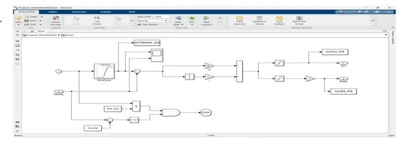
Driver model block, which is a basic PI controller that generates accelerator and brake pedal outputs to match the desired and actual vehicle speeds. The PI controller control the error between the required drive cycle and actual vehicle speed by providing acceleration and brake pedal output to the controller.

Controller Model:

The controller block is the brains of the vehicle, representing the electronic controls units. Based on the driver inputs, it generates desired engine torque, desired transmission gear and desired brake torque. These inputs are fed to the Powertrain block which represents the drivetrain of the vehicle.

A state flow machine is used to represent the supervisory control unit which decided the operating mode while it is start /stop mode or cruising mode or regen braking mode for each modes the engine drive and the motor drive are controlled.

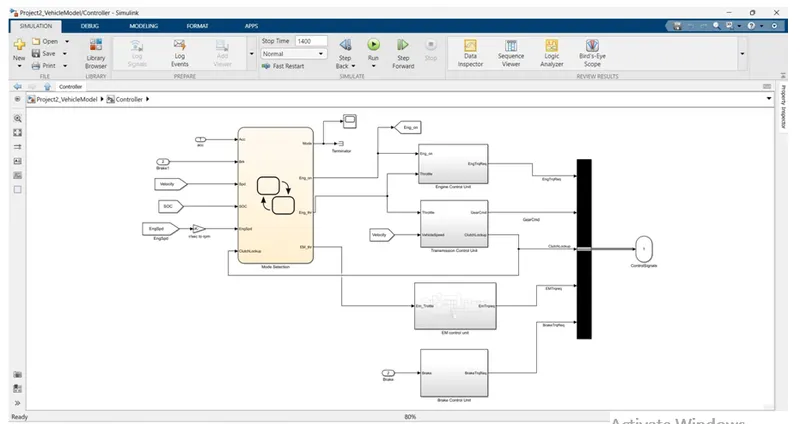
The input to the state flow charts is acceleration. and brake pedal input from the driver unit engine actual speed actual vehicle speed soc status ant the clutch lockup state and the output to the controller are the mode engine on /off request engine input throttle and electric motor input throttle.

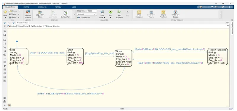
all control signal passed to transmission model which represent the drive train.

In this we created four conditions as stop, start, drive and regeneration braking. The initial block represents the stop condition. In which the engine is OFF. The engine and motor throttle conditions are zero. Then the second block represent start condition. In which the mode is 1 the electric motor throttle is only used to provide the required torque and power to the vehicle the engine is off and engine throttle conditions zero.

The state 1 and state 2 are connected using the links so, it moves from state 1 to state 2 when acceleration is less than one or SOC is less than the minimum SOC. State 3 represents mode 2 so engine is on and the engine throttle is also having positive value from the driver but the electric motor throttle is zero. It changes from state 2 to state 3 when engine speed is greater than or equal to engine idle speed. state 4 represents regenerative braking.

Engine control unit:

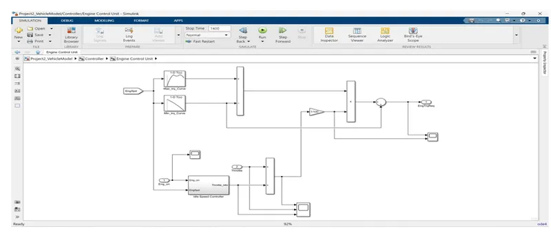
Engine control unit compare engine speed with the maximum torque and minimum torque curve of the lookup table and give the required torque command to the engine block. the throttle input is combined with the idle speed throttle and gains with torque output from the lookup table to estimate the torque input required for the engine. Throttle input idle throttle and their sum can be scoped from this block.

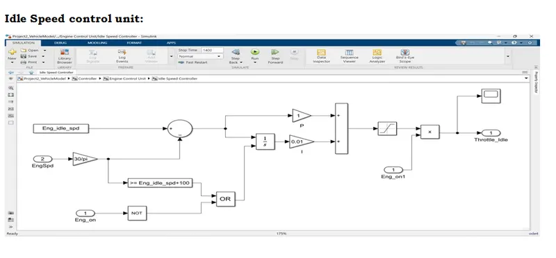
Idle Speed control unit:

Transmission control block:

The transmission control block control the gear shifting using the study flow variable chart. the gear shifting is controlled according to the vehicle speed and throttle input. the gear command is passed to the transmission block to select the desired gear ratio.

Electric motor control unit:

Motor control unit compare EM speed with the max torque curve and max torque generation curve of the lookup table and give the required torque command to the electric motor the EM throttle input is used to compare the lookup table and to estimate the torque input required for the e-motor.

Brake control Unit:

Brake control unit produce required brake torque according to the brake pedal input and passes the brake torque in to the wheel block in the transmission model.

Powertrain Model:

The power train model includes all the components that converts the power of the engine into the vehicle motion. This includes the engine, e-motor, battery pack, transmission, differential, wheels, and vehicle body dynamics subsystem.

Battery Model:

Battery pack subsystem is created with electric power input and battery soc as output. 2 diff. subblock have been created to determine the soc and terminal voltage separately soc is used to determine he terminal voltage.

SOC Estimation model:

Pack current in ampere is converted to amp-hr and divides with max capacity and adds with the initial soc to determine the soc of the battery at each instance the soc value is limited between 0 to 1.

Terminal voltage model:

Ideal voltage and internal resistance are determined by 1D lookup table and battery voltage is determined using the model. The specified values are send back to workspace using the to workspace block and can be used for post processing.

Engine model:

Based on the engine speed the required torque from the controller is saturated between max torque curve and min torque curve and passes the engine torque to the transmission block. The 2D lookup table is used to calculate the fuel flow rate based on engine speed and engine torque. The new engine also has an on/off feature to eliminate the fuel flow rate when the engine is off also the engine torque cannot be negative torque as min. torque curve mode saturated. The fuel rate is then integrated to find the fuel consumption. estimated fuel flow rate fuel consumption engine torque and engine speed are passed to the MATLAB workspace using the to-workspace block. Engine fuel flow rate and fuel consumption are scoped.

Electric motor model:

Based on the engine speed the required EM torque from the controller is saturated between max EM torque curve and max EM torque generation curve and passes the EM torque to the crank hub. The 2D lookup table is used to calculate the input electric power to the motor based on the EM speed and EM torque.

Crank Hub:

Crank hub adds up the EM torque and the engine torque and pass it to the transmission block as the crank torque.

Transmission model:

The engine block is connected to the automatic transmission via a torque converter the output of the transmission is connected to the differential.

Torque converter:

The gear selection from the transmission control unit is multiplied by the engine torque in this block and the efficiency and engine dynamics of the torque converter are applied in this model.

Differential Model:

The transmission output torque is multiplied by the differential ratio and differential efficiency in this block and the torque is transmitted to the wheel as the axle torque.

Wheel Model:

The brake torque from the control model is subtracted from the axle torque and divides from the rolling radius to determine the tractive force. The wheel speed is calculated from the vehicle velocity and saved in the workspace.

Vehicle dynamics:

The longitudinal dynamics of the vehicle along with the road load is represented in the vehicle dynamics block. Tractive force and road loads are used to calculate the vehicle velocity.

the dynamic equation for calculating road load is

M_eq(dV_veh/dt) = [(η_t*λ_tot)/(R_w)] *T_m− [0.5*ρ*A*C_d*(V_veh+V_wnd) ^2+C_r*M*g*cos(θ)+M*g*sin(θ)]

Where:

ρ = air density [kg/m^3]

A = Frontal area [m^2]

C_d = drag Co-efficient

V_veh = velocity of vehicle [m/s^2]

V_wnd = velocity of wind [m/s^2]

Cr = rolling resistance Co-efficient

M = mass in [Kg]

g = gravity.

Then we calculate and integrate then we meet acceleration of vehicle and velocity of vehicle it means vehicle distance and vehicle speed.

Plot processing MATLAB Code:

%%%%%%%%%%%%%%%%%%%%%%%%%%%%%%%%%%%%%%%%%%%%%%%%%%%%%%%%%%%%%%%%%%%%%

%% Skill-Lync -> Hybrid Drives Development

% Project 1 - Conventional Vehicle Model

% By - Ch. Venkata Sureshbabu

% Description:

% The following file is to use with the Initialization file and Simulink

% Results for post-processing of the data.

% The file is incomplete, has some examples of how the data is imported

% Into a readable format, data analysis and plotting examples.

% Based on the project task, use commands in a similar format as given

% Below, to analyse the data and generate required plots.

% You can change variable names if desired

%% Post-Processing File

% File for post-processing the Conventional vehicle simulation model data

%% Renaming variables

Time = out.tout;

Acc_Pdl = out.Acc_Pdl; % Accelerator pedal [%]

Brk_Pdl = out.Brk_Pdl; % Brake pedal [%]

Gear_Cmd = out.Gear_Cmd; % Transmission gear

Trans_In_Spd = out.Trans_In_Spd*30/pi; % Transmission input speed [rpm]

Trans_Out_Spd = out.Trans_Out_Spd*30/pi;% Transmission output speed [rpm]

Eng_Trq = out.Eng_Trq; % Engine brake torque [Nm]

Eng_Spd = out.Eng_Spd*30/pi; % Engine speed [rpm]

Eng_Fuel_Consump = out.Eng_Fuel_Consumption; % Engine fuel consumption [g]

Veh_Dist = out.Veh_Dist/1000; % Distance traveled by vehicle [km]

Veh_Spd = out.Veh_Spd*18/5; % Vehicle speed [kmph]

Wheel_Speed = out.wh_speed; % Wheel Speed [kmph]

Eng_Fuel_Rate = out.Eng_Fuel_Rate; % Engine fuel rate [%]

Desired_spd = out.Desired_spd*18/5; % cycle speed in Kmph.

%% Electric Motor varibles.

EM_Speed = out.EM_Spd; % Electical Motor Speed

EM_Power = out.EM_Pwr; % Electical Motor Power

EM_Torque = out.EM_Trq; % Electical Motor Torque

Term_Volt = out.term_volt; % Terminal Voltage of Battery

SOC = out.SOC; % State of charge

Pack_Current = out.Pack_Current; % Pack Current of Battery

WheelSpd = (Veh_Spd.*60)./(2.*pi.*Rw); % Wheel rpm

%% Data Analysis

Eng_Pwr = Eng_Spd.*pi/30.*Eng_Trq/1000; % Engine brake power [kW]

rho_petrol = 0.7197; % Density of petrol [kg/L]

kmpl = Veh_Dist(end)/(Eng_Fuel_Consump(end)/1000/rho_petrol); % Fuel economy [kmpl]

%% Plotting vehicle characteristics time trace transmission IN/OUT and wheel Speed

figure(1)

hold on

grid on

subplot(3,1,1)

plot(Time, Eng_Spd, 'linewidth', 1, 'Color', 'black');

ylabel('Eng Speed');

xlim([0, Time(end)]);

legend('Eng_Spd');

subplot(3,1,2)

hold on;

plot(Time, Trans_In_Spd, 'linewidth', 1, 'Color', 'black');

plot(Time, Trans_Out_Spd, 'linewidth', 1, 'Color', 'red');

ylabel('Speed in rpm')

xlim([0, Time(end)]);

ylim([0, 6000]);

legend('Trans Input','Trans Output');

subplot(3,1,3)

plot(Time, Wheel_Speed, 'linewidth', 1, 'Color', 'blue');

xlim([0, Time(end)]);

xlabel('Time in sec');

ylabel('Wheel Speed in kmph');

legend('Wheel Speed');

%% Plotting Engine speed, Engine Torque, Engine Power,Engine fuel rate,Engine fuel consumption wrt Time

figure(2)

subplot(4,1,1)

plot(Time,Eng_Trq,'linewidth',1,'color','black')

xlabel('Time in Sec')

ylabel('Torque in N-m')

legend('Engine Torque')

grid on

subplot(4,1,2)

plot(Time,Eng_Pwr,'linewidth',1,'color','blue')

xlabel('Time [s]')

ylabel('Power [KW]')

legend('Engine Power')

grid on

subplot(4,1,3)

plot(Time,Eng_Fuel_Rate,'linewidth',1,'color','red')

xlabel('Time in Sec')

ylabel('Fuel Rate [%]')

legend('Engine Fuel Rate')

grid on

subplot(4,1,4)

plot(Time,Eng_Fuel_Consump,'linewidth',1,'color','green')

xlabel('Time in sec')

ylabel('Fuel Consumption')

legend('Engine Fuel Consumption')

grid on

%% Plotting accelerator and brake pedal, gear command, vehicle desired and actual speed, vehicle distance using subplots.

figure(3)

subplot(5,1,1)

hold on

plot(Time, Acc_Pdl, 'linewidth', 1, 'Color', 'black');

plot(Time, Brk_Pdl, 'linewidth', 1, 'Color', 'red');

ylabel('Pedal [%]')

xlabel('Time [s]');

xlim([0, Time(end)]);

grid on

legend('Accel','Brake');

title('Acceleration & Brake Pedal w.r.t Time')

subplot(5,1,2)

plot(Time, Gear_Cmd, 'linewidth', 1, 'Color', 'black');

xlim([0, Time(end)]);

xlabel('Time [s]');

ylabel('Gear');

grid on

title('Gear command w.r.t Time')

subplot(5,1,3)

plot(Time, Veh_Spd, 'linewidth',1);

legend('Actual Spd')

title('Actual Speed of Vehicle');

xlim([0, Time(end)]);

xlabel('Time [s]');

ylabel('Speed [kmph]');

subplot(5,1,4)

plot(Time, Desired_spd, 'linewidth',1);

title('Desired Speed of Vehicle');

legend('Desired Speed')

xlim([0, Time(end)]);

xlabel('Time [s]');

ylabel('Speed [kmph]');

subplot(5,1,5)

plot(Time, Veh_Dist, 'linewidth',1);

title('Vehicle Distance')

legend('Distance');

xlim([0, Time(end)]);

xlabel('Time [s]');

ylabel('Distance [km]');

%% Plotting engine operating points on engine fuel map

figure('Name','Engine Operating Points');

hold on

grid on

title('Engine Operating Points','fontsize',12);

p1=plot(Eng_map_spd*30/pi,Eng_max_trq,'linewidth',2,'color','r');

p2=line([Eng_map_spd(end)*30/pi Eng_map_spd(end)*30/pi],[0 Eng_max_trq(end)]);

set(p2,'linewidth',1,'linestyle','--','color','k');

p3=line([Eng_map_spd(1)*30/pi Eng_map_spd(1)*30/pi],[0 Eng_max_trq(1)]);

set(p3,'linewidth',1,'linestyle','--','color','k');

[c,h] = contour(Eng_map_spd'*30/pi,Eng_map_trq,Eng_fuel_map');

clabel(c,h);

xlabel('Engine Speed [rpm]');

ylabel('Engine Torque [Nm]');

title('Engine Fuel Consumption Map [g/s]');

p4 = plot(Eng_Spd,Eng_Trq,'.','color','k');

legend([p1 p4],{'Max Curve','Operating Points'});

axis([Eng_map_spd(1)*30/pi Eng_map_spd(end)*30/pi 0 Eng_map_trq(end)]);

%% plotting motor speed, torque, motor input power using subplots.

figure(5)

subplot(3,1,1)

plot(Time, EM_Power, 'linewidth',2);

xlim([0, Time(end)]);

xlabel('Time [s]');

ylabel('power [w]');

legend('Electric Motor Power');

grid on

subplot(3,1,2)

plot(Time, EM_Torque, 'linewidth',2);

xlim([0, Time(end)]);

xlabel('Time [s]');

ylabel('Torque [Nm]');

legend('Electric Motor Torque');

grid on

subplot(3,1,3)

plot(Time, EM_Speed, 'linewidth',2);

xlim([0, Time(end)]);

xlabel('Time [s]');

ylabel('Speed [rpm]');

legend('Electric Motor Speed');

grid on

%% Plotting pack voltage, current and SoC using subplots.

figure(6)

subplot(3,1,1)

plot(Time, Pack_Current, 'linewidth',1);

xlim([0, Time(end)]);

xlabel('Time [s]');

ylabel('Current [amps]');

legend('Pack Current');

grid on

subplot(3,1,2)

plot(Time, SOC, 'linewidth',1);

xlim([0, Time(end)]);

xlabel('Time [s]');

ylabel('Charge [%]');

legend('State of Charge');

grid on

subplot(3,1,3)

plot(Time, Term_Volt, 'linewidth',1);

xlim([0, Time(end)]);

xlabel('Time [s]');

ylabel('Voltage [V]');

legend('Terminal Voltage');

grid on

%% Plotting the motor operating points on the motor input power map, with the motor max motoring and generating torque curves.

figure('Name','Electric Motor Operating Points');

hold on

grid on

title('Electric Motor Operating Points','fontsize',12);

p1=plot(EM_map_spd*30/pi,EM_max_trq,'linewidth',2,'color','r');

p2=line([EM_map_spd(end)*30/pi EM_map_spd(end)*30/pi],[0 Eng_max_trq(end)]);

set(p2,'linewidth',1,'linestyle','--','color','c');

p3=line([EM_map_spd(1)*30/pi EM_map_spd(1)*30/pi],[EM_max_gen_trq(1) Eng_max_trq(1)]);

set(p3,'linewidth',1,'linestyle','--','color','k');

[c,h] = contour(EM_map_spd'*30/pi,EM_map_trq,EM_inpwr_map');

clabel(c,h);

xlabel('Motor Speed [rpm]');

ylabel('Motor Torque [Nm]');

title('Motor Input Power Map');

p4=plot(EM_map_spd*30/pi,EM_max_gen_trq,'linewidth',1,'color','b');

legend({'Max Curve','Regen Curve','Operating Points'});

axis([EM_map_spd(1)*30/pi EM_map_spd(end)*30/pi EM_max_gen_trq(1) EM_map_trq(end)]);

Tabulate the fuel economy numbers (kmpl) for UDDS and HWFET cycle. Compare these numbers with the baseline numbers for conventional vehicle model from Project 1.

P1 HEV values of KMPL (project-2)

As per UDDS: As per HWFET

Conventional vehicle values of KMPL (project-1)

As per UDDS: As per HWFET

As we see the fuel economy number is high in HWFET when compared to UDDS cycle. Because in urban driving the vehicle encounters more traffic and it has to stop for small distance and it consumes more fuel.

As we see the fuel economy number for project 2 is little bit higher than the project 1. Because of implementing the electric motor as it is P1 hybrid vehicle. It may not much

Result plots:

1.Plot the time trace for engine, transmission input, transmission output and wheel speed on one plot.

This first plot is for time trace for engine speed, transmission input speed, transmission output speed. From this plot we see the transmission input speed is always high and wheel speed is low when compared to input speed this is happen from the units present between this two. The transmission loss and the differential loss are the reason for this variation.

UDDS:

HWFET:

2.Plot engine torque, engine power, fuel rate and fuel consumption using subplots.

The drive cycle velocity for HWFET is more in the higher range than the UDDS. The power requirement is directly proportional to the power of three for the aerodynamic drag and directly proportional to the rolling and grading resistance. Since, the proportion of higher velocity is more predominant in HWFET the vehicle requires more power to run HWFET than UDDS which means that, the fuel consumption of UDDS is less than HWFET even through the drive cycle time is more for UDDS.

UDDS:

HWFET:

3. Plot accelerator and brake pedal, gear command, vehicle desired and actual speed, vehicle distance using subplots.

The UDDS drive cycle seems to have more prominent varying velocity over time than HWFET. Therefore, more brake pedal has to be used for UDDS than HWFET which can be observed from the first subplot. The more the brake pedal is pressed. the more will be the energy loss, which in turn means that less will be the fuel economy number.

The second plot is showing the current gear position of the vehicle as the required speed it changes the gear automatically by the automatic transmission system present in this system. Third plot is shows that the current velocity of the vehicle.

UDDS:

HWFET:

4. Plot the engine operating points on the engine fuel map.

UDDS:

HWFET:

5. Plot motor speed, torque, motor input power using subplots.

This plots for the motor speed and the torque. this electric motor used in low-speed drive conditions as we mentioned in the mode logic unit. so, at the urban drive has lot of low-speed drive so it used lot of motor power in UDDS cycle when compare to HWFET cycle as shown in the plots.

UDDS:

HWFET:

6. Plot pack voltage, current and SoC using subplots.

This plot is for the pack current and the SOC. The red curves are the regen braking due to this the brake energy is converted into electrical energy and store in the battery. The second subplot shows the state of charge with the time trace.

UDDS:

HWFET:

in pdf

7. Plot the motor operating points on the motor input power map, with the motor max motoring and generating torque curves.

UDDS:

HWFET:

CONCLUSION:

Therefor the forward energy-based fuel consumption model of a P1 Hybrid vehicle has been successfully simulated using MATLAB and SIMULINK.

Analysis and understand vehicle operating points based on engine speed, torque, transmission speed, pedal position, gear, distance, velocity, acceleration, battery, voltage, current, SOC and pedal position.

Post process calculation were performed and the required graphs were successfully plotted.

Successfully calculated vehicle fuel efficiency number[kmpl] for the given city cycle [UDDS] and highway cycle [HWFET].and also compared to the conventional vehicle.