Project 2

Answers:

%% Vehicle Parameters
M = 1500;       % Vehicle weight [kg]
Cr = 0.015;     % Rolling resistance coefficient
Rw = 0.35;      % Rolling radius [m]
Cd = 0.33;      % Drag coefficient
Af = 2;         % Frontal area [m2]
rhoa = 1.225;   % Air density [kg/m3]
Vwind = 0;      % Wind velocity [kmph]
g = 9.81;       % Gravitational acceleration [m/s2]
theta = 0;      % Slope [deg]
myu_road_tire = 1; % Coefficient of friction between tire - road interface

%% Powertrain Parameters 
FDR = 3.73;                         % Final Drive Ratio / Diff Ratio
DiffEff = 0.99;                     % Differential efficiency (assumed independent of operating conditions)

NumGear = 4;                        % Number of gears in transmission
TransGear = [1:NumGear];            % Transmission Gears
TransRatio = [3.06, 1.62, 1, 0.7];  % Corresponding Transmission ratios
TransEff = 0.90;                    % Transmission efficiency (assumed independent of operating conditions)

TC_SR = [0, .5, .6, .7, .8, .87, .92, .94, .96, .97, 1];   % Torque Converter Speed Ratio (Matlab default) -> TurbSpd/PumpSpd  
TC_TR = [2.232, 1.5462, 1.4058, 1.2746, 1.1528, 1.0732, 1.0192, 1, 1, 1, 1];   % Torque Converter Torque Ratio (Matlab default) -> TurbTrq/PumpTrq
TC_Cf = 1e-4 * [.72558, .66322, .63463, .59042, .51331, .4144, .29287, .22444, .12186, .04386, 0]; % Torque Converter Capacity Factor (Matlab default) -> PumpTrq/PumpSpd^2 [Nm/rpm^2]

load Vehicle_Data/Engine_data_1_9L_Saturn_95kW
load Vehicle_Data/Trans_Shift_map
load Vehicle_Data/EM_Honda_Insight_10kW
load Vehicle_Data/ESS_NiMH6


ESS_init_soc = 0.8;
ESS_soc_max = 0.9;
ESS_soc_min = 0.6;


%% Driver Parameters
Kp = 10;                    % P gain for driver PI model
Ki = 1;                     % I gain for driver PI model
Drive_Cycle_Select = 2;     % Drive cycle selection

% Drive cycle values in m/s

if Drive_Cycle_Select == 1
    load DriveCycles/UDDS;
    
elseif Drive_Cycle_Select == 2
    load DriveCycles/HWFET;
    
elseif Drive_Cycle_Select == 3
    load DriveCycles/FTP;
    
elseif Drive_Cycle_Select == 4
    load DriveCycles/US06;
    
elseif Drive_Cycle_Select == 5
    load DriveCycles/NEDC;
    
elseif Drive_Cycle_Select == 6
    load DriveCycles/WLTP;
 
end

time_end = cyc_time(end);
vel_end = cyc_vel(end);

Simulink Modeling:

Driver Model:

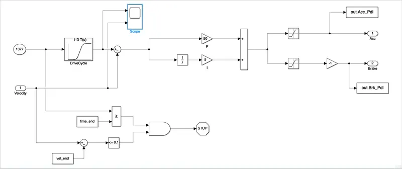
Driver Modeling is the basic generates accelerator and brake pedal output.

Controller Model:

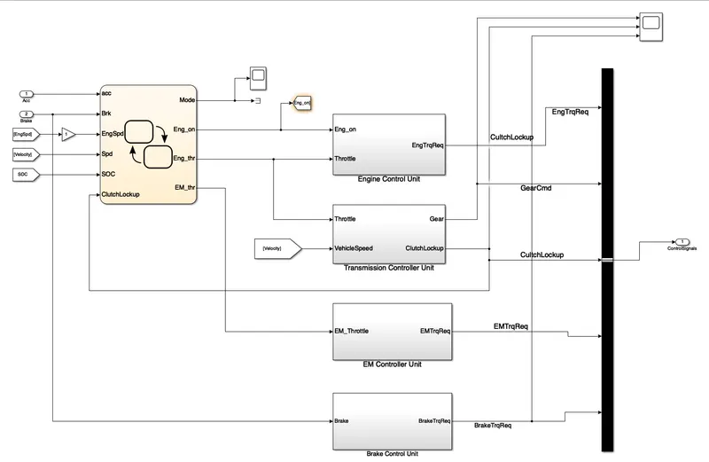
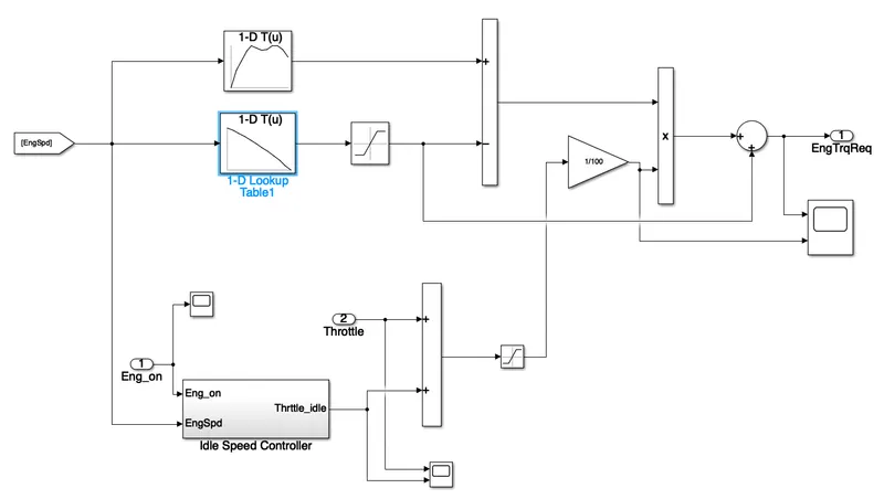
Engine control unit:

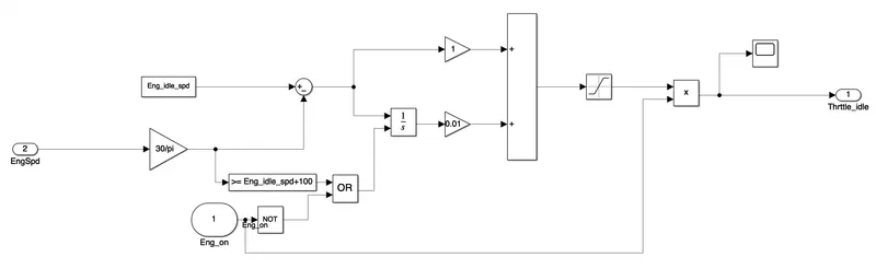
Idle speed controller:

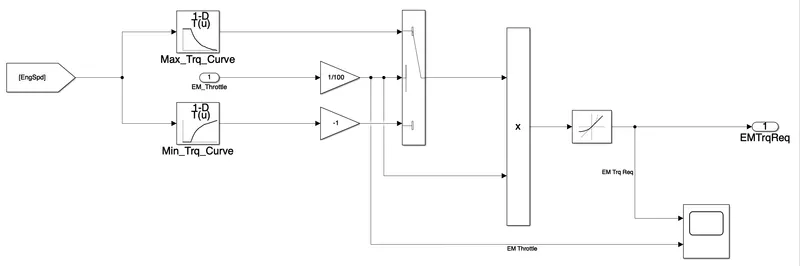
Electric motor control unit:

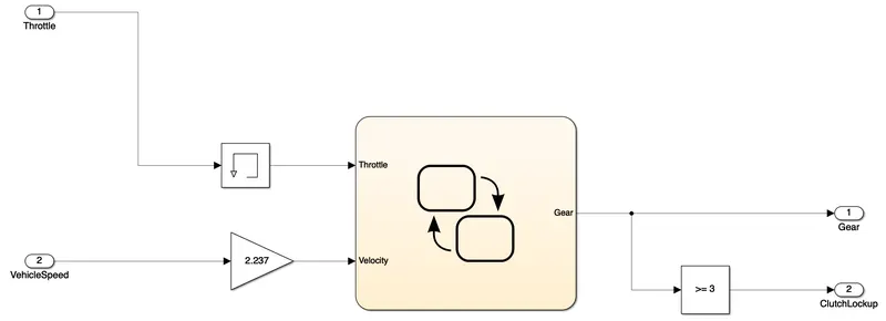
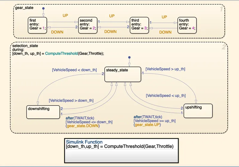
Transmission control Block:

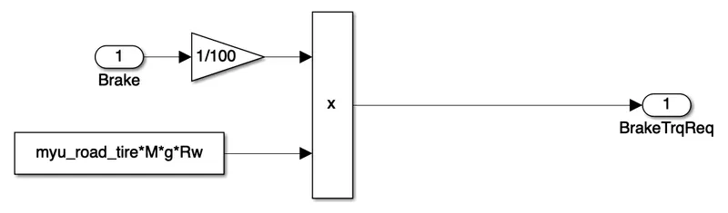
Brake control unit:

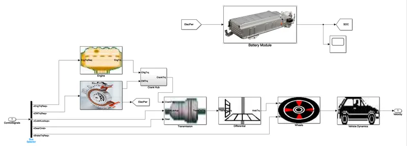
Powertrain Model:

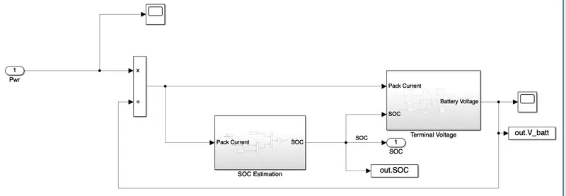
Battery Model:

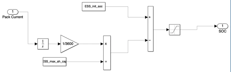
SOC Estimation model:

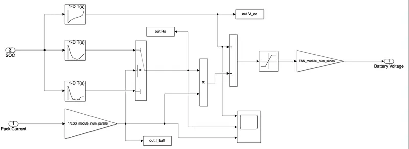
Terminal Voltage Model:

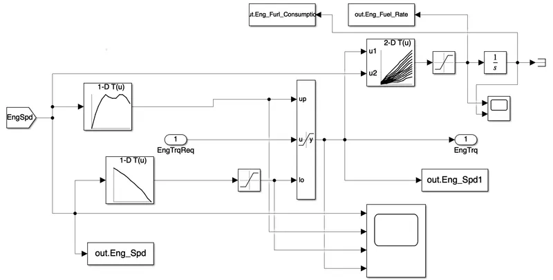
Engine Model:

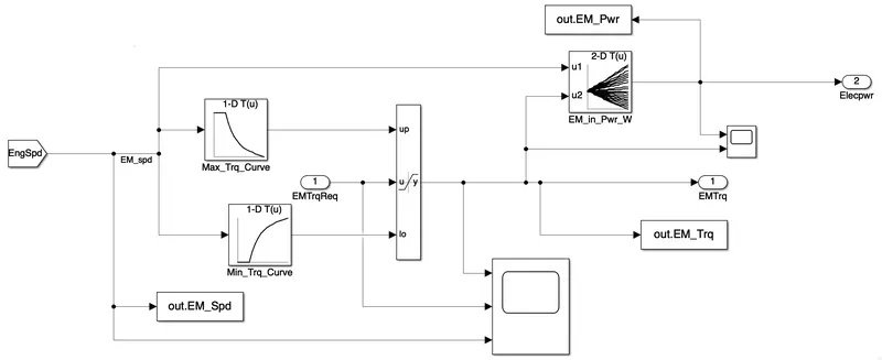
Electric motor model:

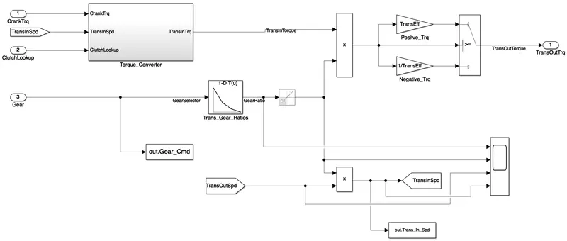
Transmission Model:

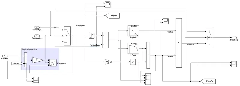
Torque Converter:

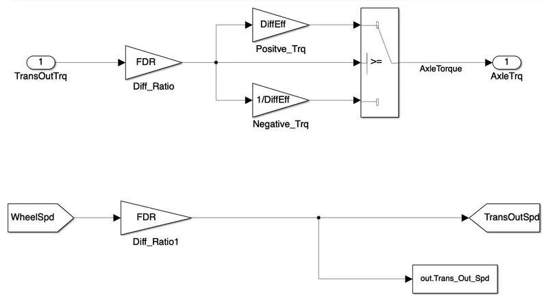
Differential Model:

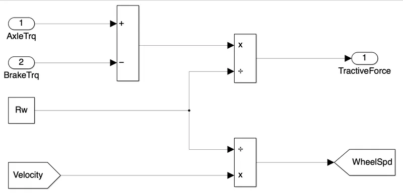
Wheel Model:

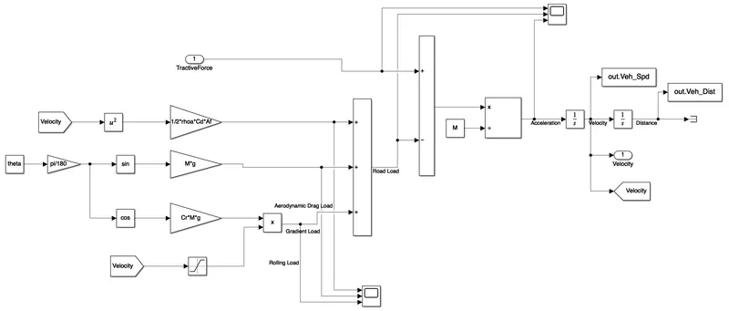
Vechile Dynamics:

RESULTS:

Drive cycle:

UDDS :

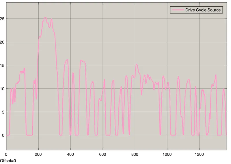
HWFET :

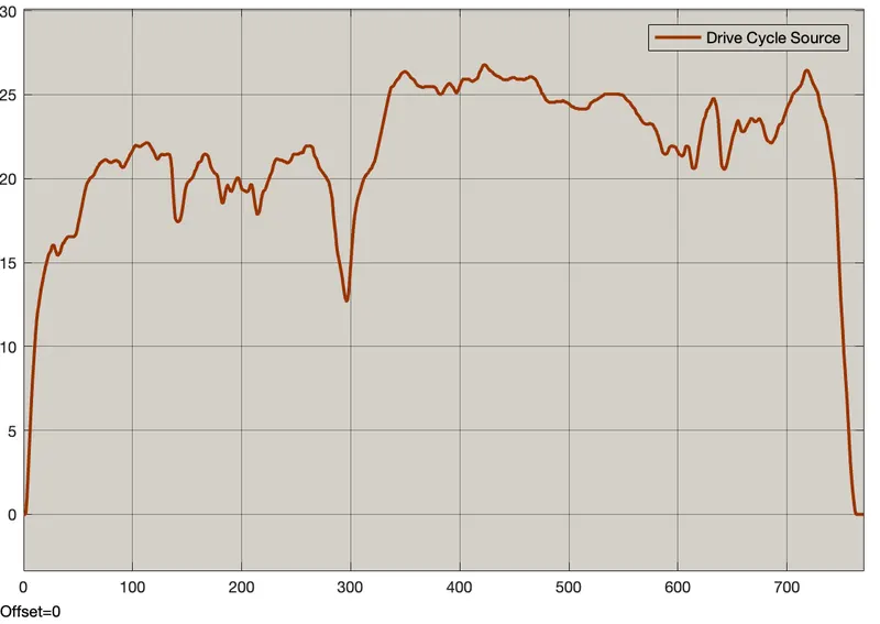
2. Fuel economy numbers (kmph) for UDDS and HWFET cycle.

UDDS :

Fuel Economy = 18.07 Kmpl

HWFET :

Fuel Economy = 22.00 Kmpl

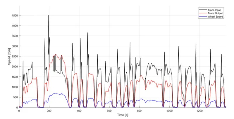
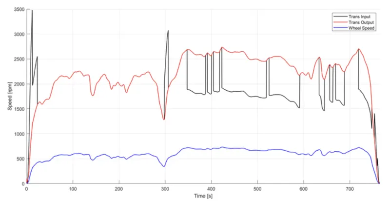
3. The Time trace for engine, Transmission input,transmission output and wheel speed

UDDS :

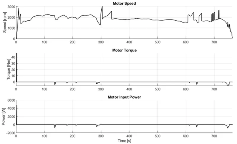
HWFET :

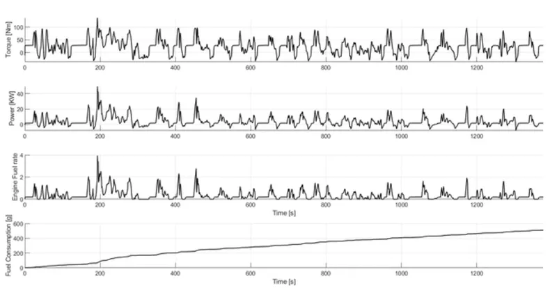
4. Engine troque, Engine power, fuel rate and fuel consumption

UDDS :

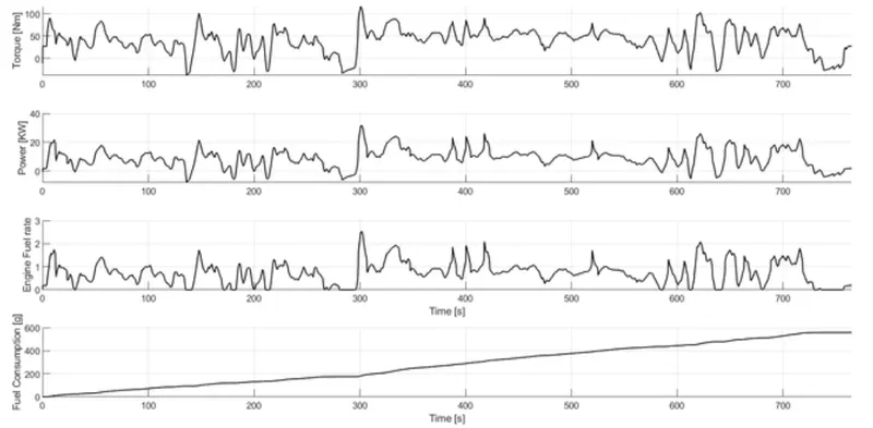
HWFET :

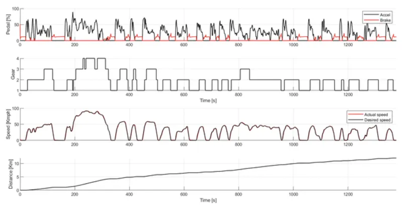
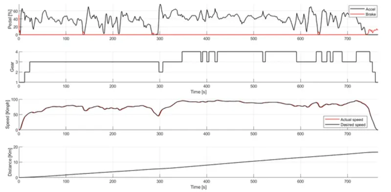
5. Accelerator and brake pedal, gear command, vehicle desired and actual speed, vehicle distance

UDDS:

HWFET:

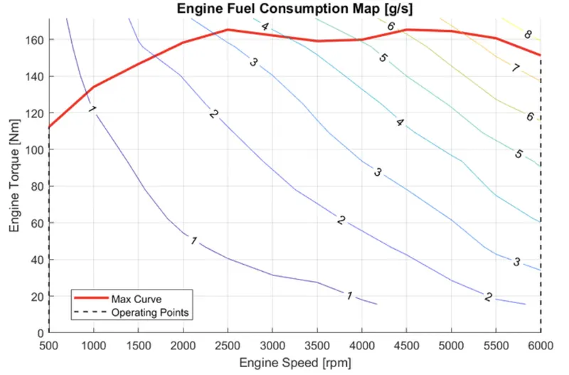
6. The engine operating points on the engine fuel map

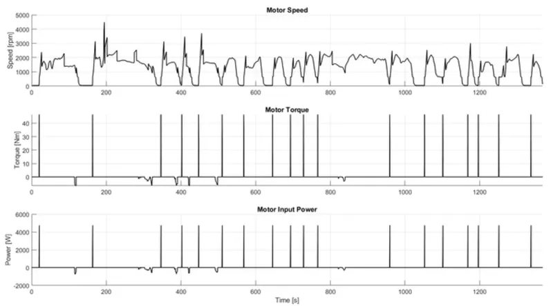
7. The Motor speed, torque, motor input power.

UDDS:

HWFET:

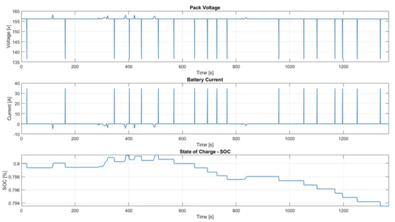
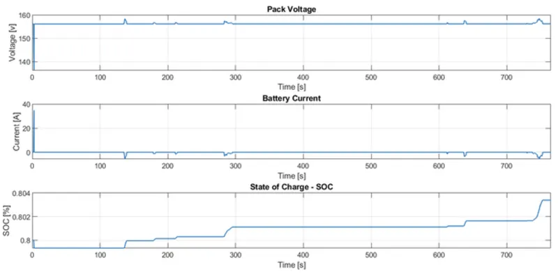
8. The Pack voltage, current and Soc

UDDS:

HWFET:

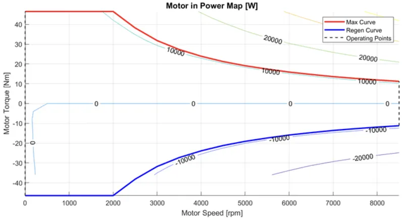
9. The motor operating points on the motor input power map, with the motor max motoring and generating
torque curves.

Conclusion:

The Various performance of characteristics and operating point of UDDS drive cycle and HWFET drive cycle are analysed and graphs are plotted.