Project 2

Aim:

• To implement clustering using an unsupervised algorithm on the car dataset
• Train a supervised model from the results obtained to predict the class of the cars

Dataset:

The dataset is about different types of cars

Number of rows:432( with empty rows in between)

Number of columns: 15

Method:

Clustering

Clustering is performed using the K-Mean algorithm, to find the right amount of clusters, the elbow plot is plotted

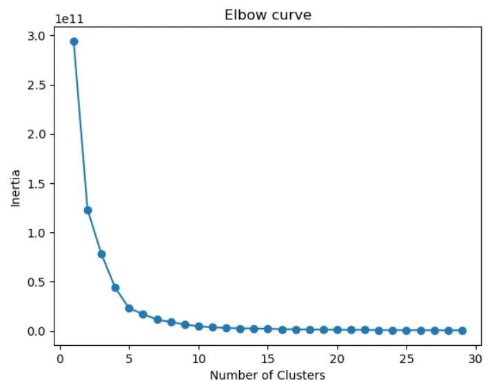
From the above plot, we can see that after 7 clusters the change in Inertia is almost zero, hence we go with 7 clusters

Results obtained from clustering

Cluster plot with respect to horsepower

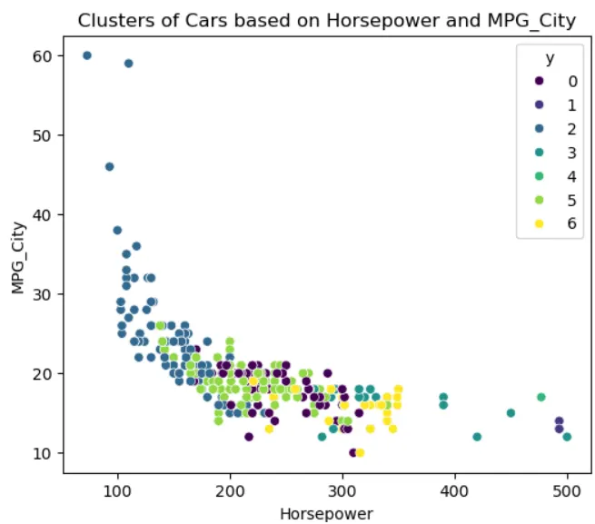
Cluster 0: Ultra-Compact, Budget Cars

• These cars are ideal for entry-level buyers, first-time car owners, or consumers in markets with a strong focus on affordability and fuel savings

Cluster 1: Standard Compact Cars (Urban Segment)

• This cluster targets urban drivers who need reliable, fuel-efficient vehicles that are easy to park and maneuver in tight spaces.

Cluster 2: Economy Family Cars

• This cluster applies to families who want a balance of affordability, fuel efficiency, and sufficient space for daily commutes and occasional trips.

Cluster 3: Mid-Range Sedans and Crossovers

• This cluster represents a versatile segment appealing to mid-level professionals, small families, or consumers who want a balance of performance, comfort, and space.

Cluster 4: Performance-Oriented Mid-Range Vehicles

• This cluster includes sporty sedans or mid-sized SUVs that applies to performance-conscious buyers who still value a degree of practicality.

Cluster 5: Luxury Cars

• This cluster represents high-income buyers looking for luxury and status. These vehicles offer advanced features, superior materials, and a smooth driving experience.

Cluster 6: High-Performance or Sports Cars

• This cluster caters to a niche market of affluent, performance-focused consumers. These are buyers who prioritize speed, power, and design over practicality or cost-efficiency.

Classification using SVM

Now the output from the clustering is used to train a supervised model, we use the support vector machine algorithm(SVM) for this purpose

Results obtained from SVM

Without prediction

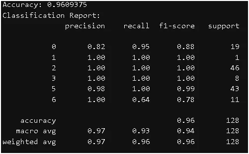
With prediction and classification report

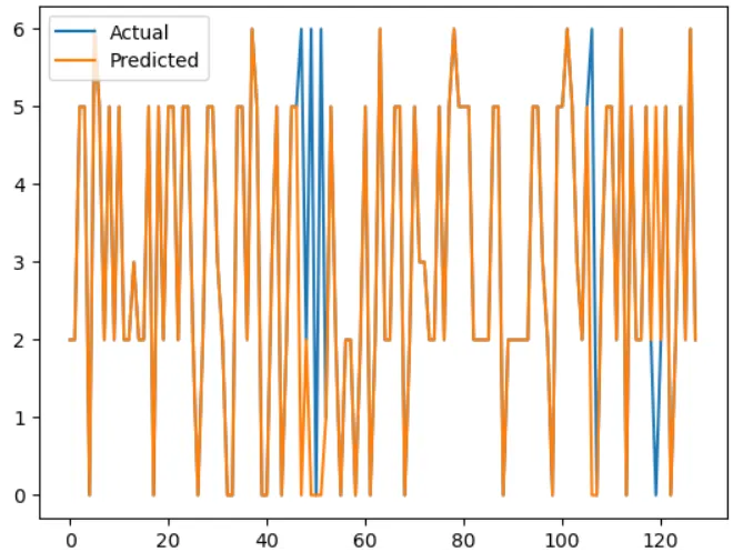
Plot between actual and predicted values

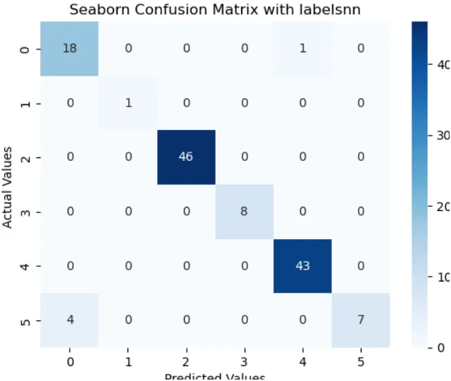
The confusion matrix is also visualized

code

# import libraries

import pandas as pd

import numpy as np

import matplotlib.pyplot as plt

import seaborn as sns

from sklearn.preprocessing import LabelEncoder

from sklearn.preprocessing import StandardScaler

from sklearn.model_selection import train_test_split

from sklearn.metrics import confusion_matrix, accuracy_score, classification_report

from sklearn.cluster import KMeans

from sklearn import svm

# load data

df=pd.read_csv('Cars Data.csv')

# First five rows

df.head()

#Total row and column

df.shape

#data info

df.info()

# Checking missing values

df.isna().sum()

#Since the missing values will not affect the clustering. So droping missing values

# droping missing values

df.dropna(inplace=True)

#checking null values

df.isnull().sum()

#Summary Statistics

df.describe().T

# Convert 'MSRP' and 'Invoice' to numeric by removing non-numeric characters

df['MSRP'] = df['MSRP'].replace(r'[\$,]', '', regex=True).astype(float)

df['Invoice'] = df['Invoice'].replace(r'[\$,]', '', regex=True).astype(float)

# converting categorical to numeric

label_encoders = {}

categorical_columns = ['Make', 'Model', 'Type', 'Origin', 'DriveTrain']

for col in categorical_columns:

le = LabelEncoder()

df[col] = le.fit_transform(df[col].astype(str))

label_encoders[col] = le

# Correlation heatmap for numeric

numeric_df = df.select_dtypes(include=['float64','int32'])

corr_matrix = numeric_df.corr()

plt.figure(figsize=(10,10))

sns.heatmap(corr_matrix, annot=True, cmap="RdYlGn")

plt.show()

#Standardizing the data

scaler = StandardScaler()

X_scaled = scaler.fit_transform(df)

#Plotting Elbow curve

from sklearn.cluster import KMeans

sse=[]

for k in range(1,30):

km=KMeans(n_clusters=k)

km.fit(df)

sse.append(km.inertia_)

plt.plot(range(1,30),sse, marker='o')

plt.title('Elbow curve')

plt.xlabel('Number of Clusters')

plt.ylabel('Inertia')

plt.show()

#KMeans Clustering

km=KMeans(n_clusters=7,random_state=0)

y=km.fit_predict(df)

#creating y column in dataframe

df['y']=y

x=df.drop(['y'],axis=1)

#dataset after addition of new column

df.head()

# Scatter plot for cluster

plt.figure(figsize=(7, 6))

sns.scatterplot(x='Horsepower', y='MPG_City', hue='y', data=df, palette='viridis')

plt.title('Clusters of Cars based on Horsepower and MPG_City')

plt.xlabel('Horsepower')

plt.ylabel('MPG_City')

plt.show()

# Pair plot for a more comprehensive view

sns.pairplot(df, hue='y', vars=['EngineSize', 'Horsepower', 'MPG_City', 'Weight','Type'])

plt.suptitle('Pair Plot of Clusters', y=1.02)

plt.show()

#Using SVM to train the model

svc=svm.SVC()

x_train,x_test,y_train,y_test=train_test_split(x,y,test_size=0.3,random_state=6)

svc.fit(x_train,y_train)

print('The training accuracy is '+str(svc.score(x_train, y_train)))

print('The test accuracy is '+str(svc.score(x_test, y_test)))

y_p=svc.predict(x_test)

accuracy = accuracy_score(y_test, y_p)

print(f'Accuracy: {accuracy}')

print('Classification Report:')

print(classification_report(y_test, y_p))

#Plot between actual and predicted values

plt.plot(y_test,label='Actual')

plt.plot(y_p,label='Predicted')

plt.legend()

plt.show()

#the confusion matrix

cf_matrix = confusion_matrix(y_test, y_p)

print(cf_matrix)

ax = sns.heatmap(cf_matrix, annot=True, cmap='Blues')

ax.set_title('Seaborn Confusion Matrix with labelsnn');

ax.set_xlabel('Predicted Values')

ax.set_ylabel('Actual Values ')

## Display the visualization of the Confusion Matrix.

plt.show()