Project 2

import pandas as pd
import numpy as np
import matplotlib.pyplot as plt
from sklearn.cluster import AgglomerativeClustering
from sklearn.preprocessing import StandardScaler
from scipy.cluster.hierarchy import dendrogram, linkage, fcluster

data = pd.read_csv('Country-data.csv', index_col=False, na_values=["?"])
df1 = pd.read_csv('Country-data.csv', index_col=False, na_values=["?"])
df = df1.copy()

features = list(df.columns)
print(features)

X1 = df[features]

X = pd.get_dummies(X1)
X = StandardScaler().fit_transform(X)

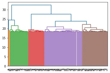
dendrogram = dendrogram(linkage(X,method='ward'))
clf = AgglomerativeClustering(n_clusters=2, affinity='euclidean', linkage='ward')
clf.fit(X)
labels = clf.labels_

data['anomaly'] = labels
outliers = data.loc[data['anomaly']==1]
outliers_index = list(outliers.index)
print(outliers_index)

print(data['anomaly'].value_counts())

from sklearn.decomposition import PCA
from sklearn.preprocessing import StandardScaler
from mpl_toolkits.mplot3d import Axes3D
pca = PCA(n_components=3)
scaler = StandardScaler()

X = scaler.fit_transform(X)
X_reduce = pca.fit_transform(X)

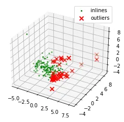
fig = plt.figure()
ax = fig.add_subplot(111, projection = '3d')

ax.scatter(X_reduce[:,0], X_reduce[:,1], zs = X_reduce[:,2], s=4, lw=1,
label="inlines", c="green")
ax.scatter(X_reduce[outliers_index,0], X_reduce[outliers_index,1],X_reduce[outliers_index,2],
lw=2, s=60, marker="x", c="red", label="outliers")
ax.legend()
plt.show()

Output

['country', 'child_mort', 'exports', 'health', 'imports', 'income', 'inflation', 'life_expec', 'total_fer', 'gdpp']
[7, 8, 11, 15, 23, 29, 44, 53, 54, 58, 60, 68, 73, 74, 75, 77, 82, 89, 91, 98, 110, 111, 114, 115, 122, 123, 128, 133, 139, 144, 145, 157, 158, 159]
0    133
1     34
Name: anomaly, dtype: int64

​