Project 2

Objective: To modify the MATLAB model of the conventional vehicle and incorporate the hybrid functionality by adding the electric motor to the model. And write a brief about the obtained results from the model and compare the result with the conventional vehicle model.

Modification:

Initiation script:

%% Vehicle Parameters
M = 1500;       % Vehicle weight [kg]
Cr = 0.015;     % Rolling resistance coefficient
Rw = 0.35;      % Rolling radius [m]
Cd = 0.33;      % Drag coefficient
Af = 2;         % Frontal area [m2]
rhoa = 1.225;   % Air density [kg/m3]
Vwind = 0;      % Wind velocity [kmph]
g = 9.81;       % Gravitational acceleration [m/s2]
theta = 0;      % Slope [deg]
myu_road_tire = 1; % Coefficient of friction between tire - road interface

%% Powertrain Parameters 
FDR = 3.73;                         % Final Drive Ratio / Diff Ratio
DiffEff = 0.99;                     % Differential efficiency (assumed independent of operating conditions)

NumGear = 4;                        % Number of gears in transmission
TransGear = 1:NumGear;            % Transmission Gears
TransRatio = [3.06, 1.62, 1, 0.7];  % Corresponding Transmission ratios
TransEff = 0.90;                    % Transmission efficiency (assumed independent of operating conditions)

TC_SR = [0, .5, .6, .7, .8, .87, .92, .94, .96, .97, 1];   % Torque Converter Speed Ratio (Matlab default) -> TurbSpd/PumpSpd  
TC_TR = [2.232, 1.5462, 1.4058, 1.2746, 1.1528, 1.0732, 1.0192, 1, 1, 1, 1];   % Torque Converter Torque Ratio (Matlab default) -> TurbTrq/PumpTrq
TC_Cf = 1e-4 * [.72558, .66322, .63463, .59042, .51331, .4144, .29287, .22444, .12186, .04386, 0]; % Torque Converter Capacity Factor (Matlab default) -> PumpTrq/PumpSpd^2 [Nm/rpm^2]

load Vehicle_Data/Engine_data_1_9L_Saturn_95kW
load Vehicle_Data/Trans_Shift_map
load Vehicle_Data/EM_Honda_Insight_10kW
load Vehicle_Data/ESS_NiMH6


ESS_init_soc = 0.8;
ESS_soc_max = 0.9;
ESS_soc_min = 0.6;


%% Driver Parameters
Kp = 10;                    % P gain for driver PI model
Ki = 1;                     % I gain for driver PI model
Drive_Cycle_Select = 2;     % Drive cycle selection

% Drive cycle values in m/s

if Drive_Cycle_Select == 1
    load DriveCycles/UDDS;
    
elseif Drive_Cycle_Select == 2
    load DriveCycles/HWFET;
    
elseif Drive_Cycle_Select == 3
    load DriveCycles/FTP;
    
elseif Drive_Cycle_Select == 4
    load DriveCycles/US06;
    
elseif Drive_Cycle_Select == 5
    load DriveCycles/NEDC;
    
elseif Drive_Cycle_Select == 6
    load DriveCycles/WLTP;
 
end

time_end = cyc_time(end);
vel_end = cyc_vel(end);

To achieve the hybrid functionality required data for the preparation of the lookup tables for electric motors and batteries and also various parameters for maintaining battery operating conditions are added to the initiation script.

Simulink model:

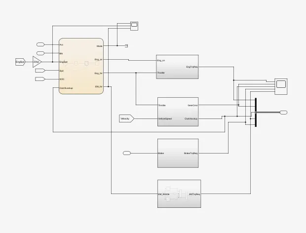
To incorporate the hybrid functionality into the conventional certain features such as supervisory control, electric motor control, electric motor, and battery.

Clutchlockup:

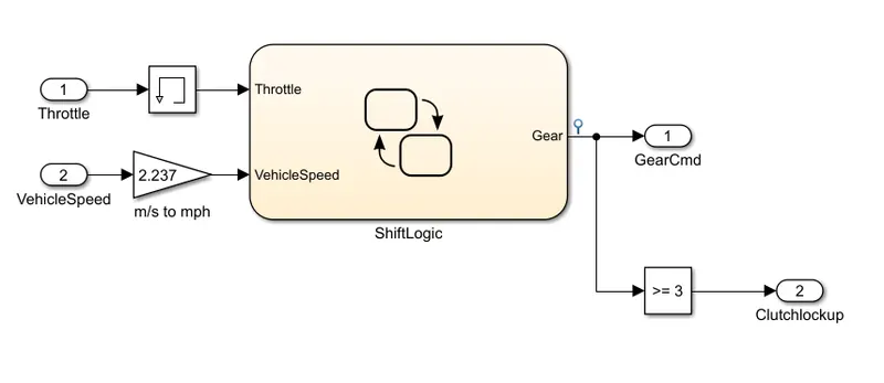
When the gear command from the user is 3 or more than 3 the turbine and pump of the torque converter are locked using a clutch to avoid transmission losses and increase the efficiency of the vehicle.

Supervisory control: In the controller block of the conventional vehicle the supervisory control state logic is added to control the engine and electric motor operating conditions.

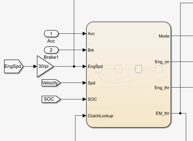
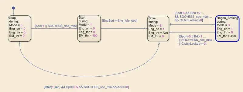
In the Stateflow, as shown in the figure above four states are created and various conditions are implemented to transition between each state.

When the model is initiated to run state 1 is activated which is when the engine is off and the values of engine throttle and electric motor throttle are zero. And if the value of the acceleration from the user is more than 1 or the State of charge of the battery is less than a minimum limit of the battery SOC specified in the model the control moves to the state 2

In state 2 electric motor throttle is fully turned to assist in the startup of the engine and add up the required torque for the quick acceleration of the vehicle.

And when the engine is greater than the mentioned idle speed of the engine the control is transferred to state 3 of the Stateflow. During this state, the electric motor is turned off and the torque is transmitted directly from the engine to the transmission without any assistance as per the acceleration requirement.

And the state control moves from state 3 to state 4 if the velocity of the engine is more than 6 and braking torque is more than 2 that is when the brakes are applied and the SOC of the battery is less than the SOC max mentioned by user and clutch is locked up in the torque convertor the regenerative braking is activated and the power of the engine during the braking is diverted to the battery pack and any of the above-mentioned conditions are invalidated the Stateflow control is transferred back to the state 3.

And also when the velocity of the vehicle is less than 0.5 and battery SOC is more than the minimum mentioned limit of the SOC and acceleration is 0 the Stateflow control from state 3 is transferred to state 1.

Engine controller:

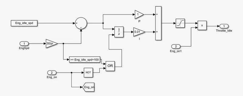
In the engine controller, the engine is turned off as per the state logic signals.

Electric motor controller:

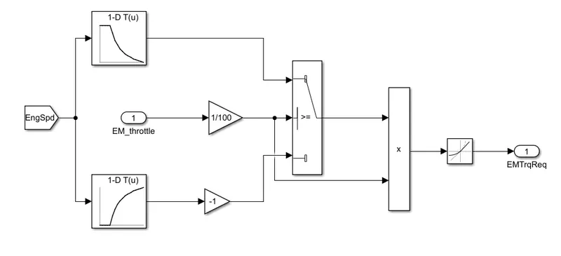
In the electric motor controller, it can be seen that the motor torque requirement is generated as per the engine speed using the 1D lookup table, and a switch block is used to decide if the torque generated is positive of regenerative torque which is to be directed to the battery and also controls the motor operation as the motor signal from the state logic is multiplied to with the output torque.

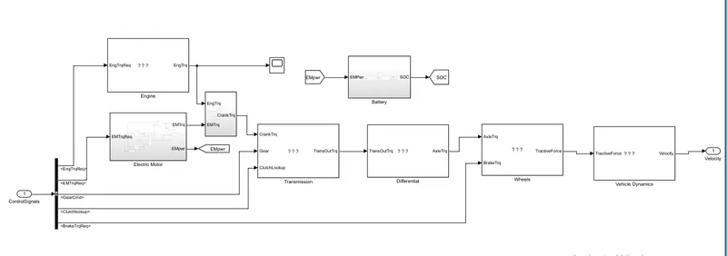
As shown in the figure above in the powertrain subsystem the electric motor, battery, and crankshaft subsystems are added to incorporate the hybrid functionality.

Engine:

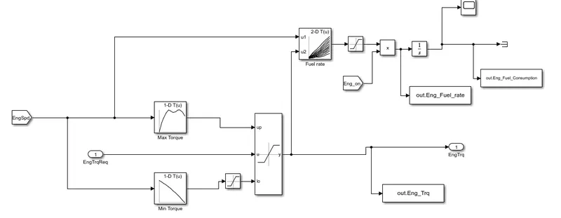In the engine, the eng on switch is added to switch the fuel output when the engine is turned off.

Electric motor:

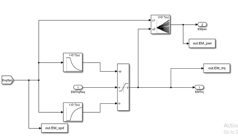
As shown in the figure the torque supplied by the electric motor is as per the engine speed and the torque requirement provided by the electric motor controller. Using a 1D lookup table referring to the engine speed the torque to be supplied by the electric motor is decided and the saturation switch is used to decide the nature of the torque i.e. positive torque to assist the engine or regenerative torque to be diverted to the battery pack.

And also the electric motor power to be supplied using the 1D lookup table referring to the engine speed.

Battery:

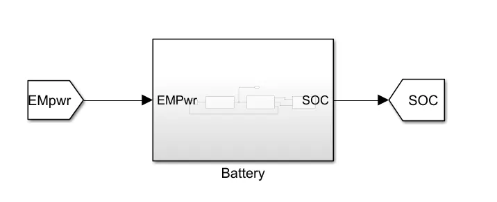
The battery subsystem modeled as a part of the previous challenge is used and as shown in the figure the electric motor power requirement is supplied to the model and the SOC of the battery is computed using the battery subsystem.

Crankshaft:

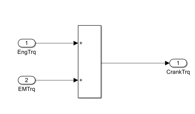
In the crankshaft subsystem, as illustrated above the torques from the engine and electric motor are coupled for better performance of the vehicle. 

Torque converter:

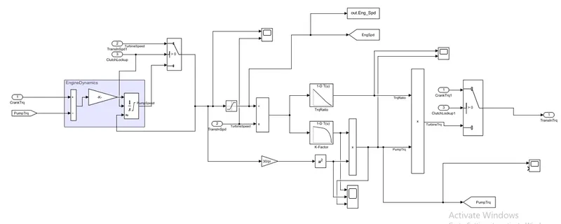
In the torque converter subsystem of the transmission, various changes are made to add the clutch lockup functionality i.e to lock the turbine and pump of the torque converter at higher speed values using the clutch. In this the values of the crank torque and pump torque are integrated over time with the feedback of the clutch lockup i.e. the integrator is reset whenever the clutch is locked and the turbine speed is directly supplied to the pump which indicates that the crank torque is directly supplied to the transmission and when there is no lock up the pump speed is taken into consideration.

Postprocessing Script:

%% Renaming variables
Time = out.tout;
Acc_Pdl = out.Acc_Pdl;                          % Accelerator pedal [%]
Brk_Pdl = out.Brk_Pdl;                          % Brake pedal [%]
Gear_Cmd = out.Gear_Cmd;                        % Transmission gear
Trans_In_Spd = out.Trans_In_Spd*30/pi;          % Transmission input speed [rpm]
Trans_Out_Spd = out.Trans_Out_Spd*30/pi;        % Transmission output speed [rpm]
Eng_Trq = out.Eng_Trq;                          % Engine brake torque [Nm]
Eng_Spd = out.Eng_Spd*30/pi;                    % Engine speed [rpm]
Eng_Fuel_Consump = out.Eng_Fuel_Consumption;    % Engine fuel consumption [g]
Veh_Dist = out.Veh_Dist/1000;                   % Distance traveled by vehicle [km]
Veh_Spd = out.Veh_Spd*18/5;                     % Vehicle speed [kmph]
Eng_Fuel_rate = out.Eng_Fuel_rate;              %Fuel consumption rate[g/s]
Veh_desire_Spd = out.Veh_desire_Spd*18/5;       %Speed of the drive cycle[kmph]
Wheel_Spd = out.Wheel_Spd*30/pi;                %Wheel Speed in [rpm]
EMpwr = out.EM_pwr;                             %Motor power in kW
EMspd = out.EM_spd*30/pi;                       %Motor speed in rpm
EMtrq = out.EM_trq;                             %Motor torque in Nm
SOC_batt = out.SOC;                             %SOC of battery
Packcurrent = out.pack_current;                 %Pack current drawn and supplied by battery in Amp
Terminal_volt = out.Term_V;                     %Terminal voltage of battery                   





%% Data Analysis
Eng_Pwr = (Eng_Spd.*pi/30).*(Eng_Trq./1000);   % Engine brake power [kW]
rho_petrol = 0.7197;                    % Density of petrol [kg/L]
kmpl = Veh_Dist(end)/(Eng_Fuel_Consump(end)/1000/rho_petrol);    % Fuel economy [kmpl] 


%% Plotting vehicle characteristics time trace
figure()
subplot(4,1,1)
hold on
grid on
plot(Time, Acc_Pdl, 'linewidth', 1, 'Color', 'black');
plot(Time, Brk_Pdl, 'linewidth', 1, 'Color', 'red');
ylabel('Pedal [%]')
xlim([0, Time(end)]);
legend('Accel','Brake');
title('Acceleration and Brake value')
subplot(4,1,2)
hold on
grid on
plot(Time, Veh_Dist)
ylabel('Distance [km]')
xlim([0, Time(end)]);
title('Distance Travelled')
subplot(4,1,4)
hold on
grid on
plot(Time, Gear_Cmd, 'linewidth', 1, 'Color', 'black');
xlim([0, Time(end)]);
xlabel('Time [s]');
ylabel('Gear');
title('Gear No.')
subplot(4,1,3)
hold on
grid on
plot(Time,Veh_Spd,'Color','r')
plot(Time,Veh_desire_Spd,'Color','k')
xlim([0, Time(end)]);
ylabel('Speed [kmph]')
title('Actual vs Desired Speed')
legend('Actual Speed','Desired Speed')

%% Plotting engine operating points on engine fuel map
figure('Name','Engine Operating Points');
hold on
grid on
title('Engine Operating Points','fontsize',12);
p1=plot(Eng_map_spd*30/pi,Eng_max_trq,'linewidth',2,'color','r');
p2=line([Eng_map_spd(end)*30/pi Eng_map_spd(end)*30/pi],[0 Eng_max_trq(end)]);
set(p2,'linewidth',1,'linestyle','--','color','k');
p3=line([Eng_map_spd(1)*30/pi Eng_map_spd(1)*30/pi],[0 Eng_max_trq(1)]);
set(p3,'linewidth',1,'linestyle','--','color','k');
[c,h] = contour(Eng_map_spd'*30/pi,Eng_map_trq,Eng_fuel_map');
clabel(c,h);
xlabel('Engine Speed [rpm]');
ylabel('Engine Torque [Nm]');
title('Engine Fuel Consumption Map [g/s]');
p4 = plot(Eng_Spd,Eng_Trq,'.','color','k');
legend([p1 p4],{'Max Curve','Operating Points'});
axis([Eng_map_spd(1)*30/pi Eng_map_spd(end)*30/pi 0 Eng_map_trq(end)]);

figure()
subplot(4,1,3)
hold on
grid on
plot(Time,Eng_Fuel_rate)
xlim([0, Time(end)]);
ylabel('Fuel Rate[gm/s]')
title('Fuel rate')
subplot(4,1,4)
plot(Time,Eng_Fuel_Consump)
hold on
grid on
xlim([0, Time(end)]);
ylabel('Fuel [g]')
xlabel('Time [s]')
title('Fuel Consumption in gm')
subplot(4,1,1)
hold on
grid on
plot(Time,Eng_Trq)
xlim([0, Time(end)]);
ylabel('Torque [Nm]')
title('Engine torque in Nm')
subplot(4,1,2)
hold on
grid on
plot(Time,Eng_Pwr)
xlim([0, Time(end)]);
ylabel('Power [kw]')
title('Engine Power in kw')

figure()
plot(Time,Trans_Out_Spd,'Color','r')
hold on
grid on
plot(Time,Trans_In_Spd,'Color','k')
plot(Time,Wheel_Spd,'Color','b')
xlim([0, Time(end)]);
ylabel('Speed [rpm]')
xlabel('Time [s]')
legend('Trans Out', 'Trans In', 'Wheel Speed')

figure()
subplot(3,1,1)
plot(Time,SOC_batt)
xlim([0, Time(end)]);
ylabel('SOC Battery')
xlabel('Time [s]')
title('State of charge')

subplot(3,1,2)
plot(Time,Packcurrent);
xlim([0, Time(end)]);
xlabel('Time [s]')
ylabel('Current [A]')
title('Battery pack current')

subplot(3,1,3)
plot(Time,Terminal_volt);
xlim([0,Time(end)]);
xlabel('Time [s]');
ylabel('Terminal voltage [V]')
title('Battery termianl voltage')

figure()
subplot(3,1,1)
plot(Time,EMspd);
xlim([0, Time(end)])
xlabel('Time [s]')
ylabel('Speed [rpm]')
title('Motor speed')

subplot(3,1,2)
plot(Time,EMtrq)
xlim([0, Time(end)])
xlabel('Time [s]')
ylabel('Torque [Nm]')
title('Motor torque')

subplot(3,1,3)
plot(Time,EMpwr);
xlim([0, Time(end)])
xlabel('Time [s]')
ylabel('Power [W]')
title('Motor Power')

figure('Name','Motor Operating Points');
hold on
grid on
title('Motor Operating Points','fontsize',12);
ylim([EM_max_gen_trq(1), EM_max_trq(end)]);
xlim([-5, EM_map_spd(end)*30/pi]);
p5=plot(EM_map_spd*30/pi,EM_max_trq,'linewidth',2,'color','r');
p1=plot(EM_map_spd*30/pi,EM_max_gen_trq,'linewidth',2,'Color','b');
p2=line([EM_map_spd(end)*30/pi EM_map_spd(end)*30/pi],[0 EM_max_trq(end)]);
set(p2,'linewidth',1,'linestyle','--','color','k');
p3=line([EM_map_spd(1)*30/pi EM_map_spd(1)*30/pi],[0 EM_max_trq(1)]);
set(p3,'linewidth',1,'linestyle','--','color','k');
xlabel('Engine Speed [rpm]');
ylabel('Engine Torque [Nm]');
p4 = plot(EMspd,EMtrq,'.','color','k');
legend([p5 p1 p4],{'Max torque Curve','Max regen curve','Operating Points'});
axis([0 EM_map_spd(end)*30/pi EM_max_gen_trq(1) EM_map_trq(end)]);

 The values from this Simulink model are transferred back to the Matlab script with the use of the To Workspace block and the postprocessing script is used to plot all the results of the vehicle as per the challenge.

Comparison of UDDS and HWFET cycle:

UDDS Plot

 

HWFET Plot

 

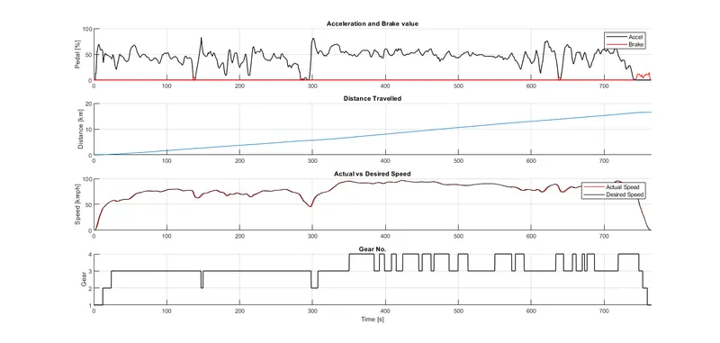
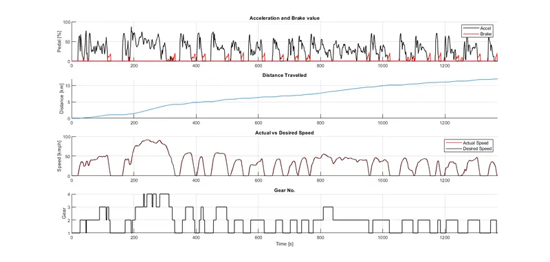
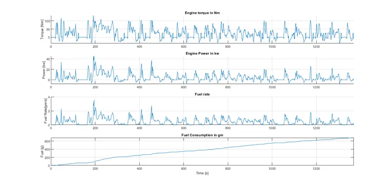
Here it can be clearly seen that the urban drive runs at lower speed and requires lower gears with higher torque ratios to fulfill its high acceleration demand compared to the highway drive cycle which has less braking conditions and runs on higher gear numbers with low torque ratios. And the vehicle in the highway drive cycle covers more distance i.e. about 16km in 800secs while the distance traveled by the vehicle in the urban drive is about 14km in 1300secs and both the vehicle uses the same quantity of the fuel i.e. 700gms of fuel which can be seen the plot no. 4 below hence the HWFET drive cycle is much more efficient compared to the UDDS cycle.

Fuel Consumption Map of UDDS cycle

Fuel Consumption Map of HWFET cycle

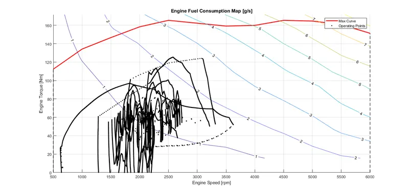
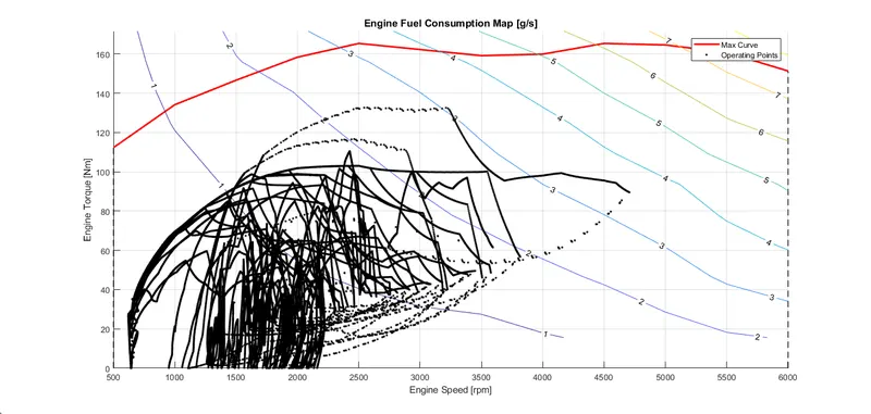
 Here from the operating points of the engine, it can be seen that the HWFET cycle consumes less fuel and performs more efficiently by operating at lower engine speeds and lower engine torque compared to the urban drive cycle which operates the engine at higher speeds and higher torque hence being less efficient and consuming more fuel.

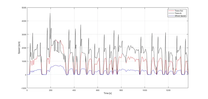
Speeds plot of the UDDS cycle

Speeds plot of HWFET cycle

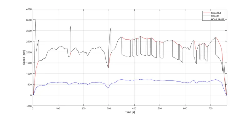
It can be seen that the transmission output speed of the highway drive cycle is higher than its transmission input speed hence less effort is required to move the vehicle forward which results in faster wheel speed, while in the urban drive cycle the transmission output speed is lower than the transmission output speed so more effort is required to move the vehicle forward and so the wheels move at a lesser speed.

UDDS Cycle plot

HWFET cycle plot

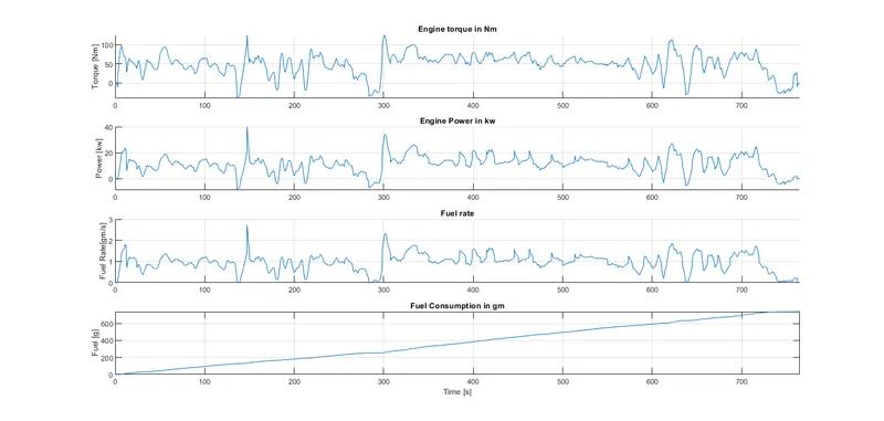
In the above plot, it can be seen that the operating power and torque of the engine in the highway drive cycle are less compared to the urban drive cycle and the fuel consumption of both cycles is almost equal at 700gms but the distance traveled by the vehicle in the highway is about 16km and that in the urban drive cycle is about 14km in higher time span this indicates that the efficiency of the highway drive cycle is far better than the urban drive cycle as it has less break torque being applied on the wheels which reduces the overall torque requirement on the engine and provide it better operating conditions to perform efficiently.

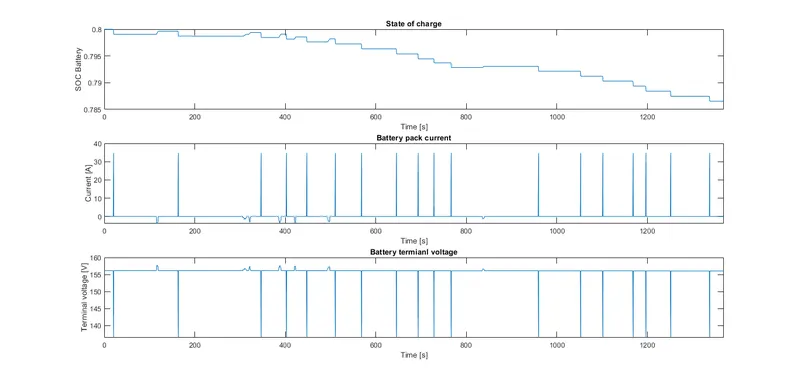
Battery parameters for UDDS cycle

Battery parameters for HWFET cycle

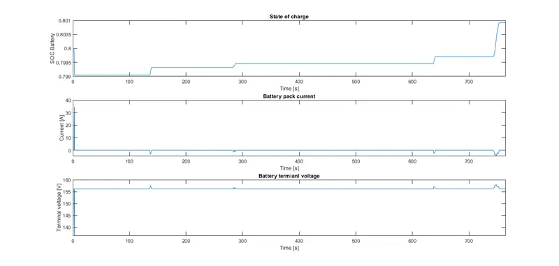
As seen from the results above during the UDDS cycle as the vehicle is required to continuously accelerate and deaccelerate the electric motor is operated frequently to assist the acceleration and as a result more power is required to power the electric motor in the UDDS cycle and so the battery SOC is decreased from 80% to 78.7% while in the HWFET cycle due to regenerative breaking the and less power requirement by the electric motor as the motor is used only during the startup of the engine and during the rest of the cycle motor is idle as the vehicle do not deaccelerate to 0 km/hr and so the battery SOC is actually increased from 80% to 80.05% after decreasing during the startup.

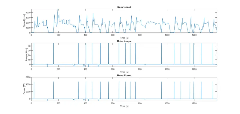
Motor parameters for UDDS cycle:

Motor parameters for HWFET cycle:

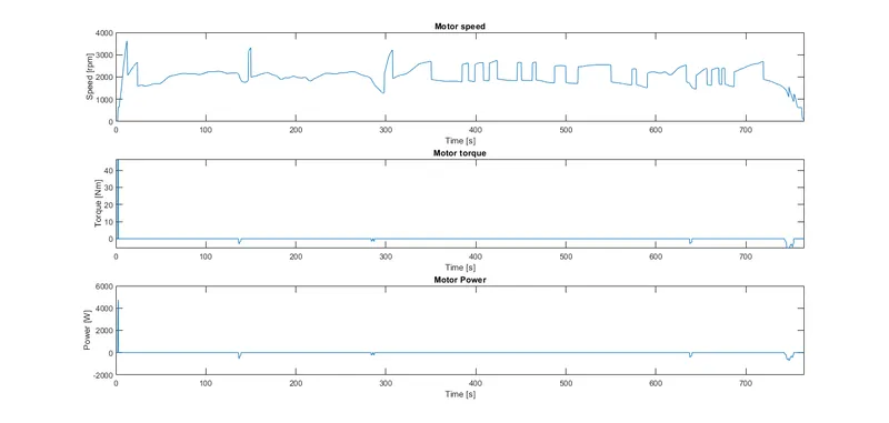
As the motor is coupled with the engine but not engaged the speed of the motor is plotted while the power generated by the motor is not. During the UDDS cycle due to constant acceleration and deacceleration to assist the engine, an electric motor is operated more frequently, while in the HWFET cycle the motor only assists the engine during the startup, and during the rest of the cycle, the motor is either ideal or generate power during braking.

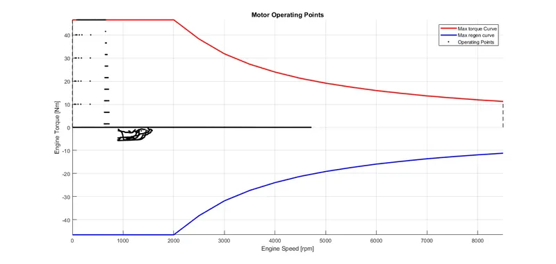
Electric motor operating points for UDDS cycle:

Electric motor operating points for HWFET cycle:

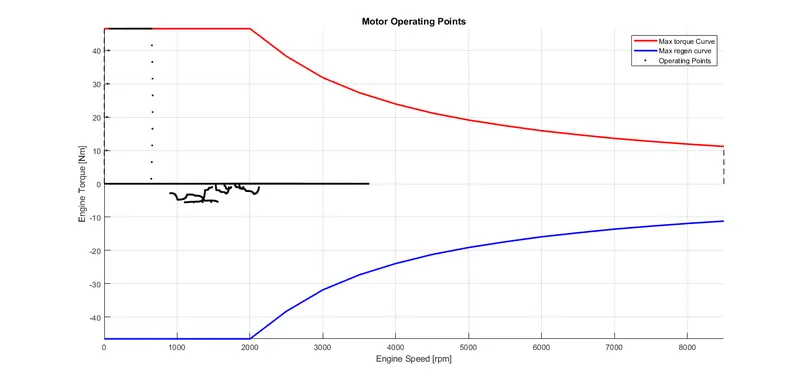
As shown in the figure, the motor operates in the left-most corner or left side at low speeds and high torque which represents that the motor only assists the engine when its speeds are low and the torque requirement is high and the negative torque operating points represent the regenerative braking.

 Comparing the fuel consumption of UDDS cycle for conventional and hybrid vehicles:

Conventional vehicle fuel consumption

Hybrid vehicle fuel consumption

As shown in the figure it can be seen that the fuel consumption of the fuel is decreased from 744.61 gms to 682.85 gms which is a decrease of about 8.29% which shows how efficient the P1 hybrid vehicles can be in the urban drive cycle.

Comparing the fuel consumption of HWFET cycle for conventional and hybrid vehicles:

Conventional vehicle fuel consumption

Hybrid vehicle fuel consumption

As shown in the figure it can be seen that the fuel consumption of the fuel is decreased from 763.55 gms to 737.20 gms which is a decrease of about 3.45% which shows that even when the P1 hybrid vehicles are used on the highway it can save significant fuel during the longer drive cycle.