Project 2

1. What is KMeans Clustering?

2. Performing KMeans Clustering.

3. What is Hierarchical Clustering and its types?

4. Performing Hierarchical clustering on the datasets.

5. Summary and Conclusion.

K-Means Clustering Algorithm:

· K-Means Clustering is an Unsupervised Learning algorithm, which groups the unlabelled dataset into different clusters. Here K defines the number of pre-defined clusters that need to be created in the process, if K=2, there will be two clusters, and for K=3, there will be three clusters, and so on.

· It is an iterative algorithm that divides the unlabelled dataset into k different clusters in such a way that each dataset belongs to only one group that has similar properties.

· It allows us to cluster the data into different groups and a convenient way to discover the categories of groups in the unlabelled dataset on its own without the need for any training.

· It is a centroid-based algorithm, where each cluster is associated with a centroid. The main aim of this algorithm is to minimize the sum of distances between the data point and their corresponding clusters.

· The algorithm takes the unlabeled dataset as input, divides the dataset into k-number of clusters, and repeats the process until it does not find the best clusters. The value of k should be predetermined in this algorithm.

The k-means clustering algorithm mainly performs two tasks:-

• Determines the best value for K centre points or centroids by an iterative process.
• Assign each data point to its closest K-centre. Those data points which are near to the particular k-centre, create a cluster.

Hence each cluster has data points with some commonalities, and it is away from other clusters.

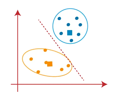
The below diagram explains the working of the K-means Clustering Algorithm:-

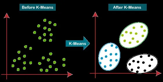
The working of the K-Means algorithm is explained in the below steps:-

Ø Select the number K to decide the number of clusters.

Ø Select random K points or centroids. (It can be other than the input dataset).

Ø Assign each data point to its closest centroid, which will form the predefined K clusters.

Ø Calculate the variance and place a new centroid of each cluster.

Ø Repeat the third step, which means reassigning each datapoint to the new closest centroid of each cluster.

Ø If any reassignment occurs, then go to step-4 else go to FINISH.

Ø The model is ready.

Let's understand the above steps by considering the visual plots:-

Suppose we have two variables M1 and M2. The x-y axis scatter plot of these two variables is given below:

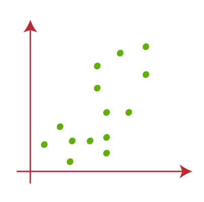
• Let's take number k of clusters, i.e., K=2, to identify the dataset and to put them into different clusters. It means here we will try to group these datasets into two different clusters.
• We need to choose some random k points or centroid to form the cluster. These points can be either the points from the dataset or any other point. So, here we are selecting the below two points as k points, which are not the

Part of our dataset. Consider the below image:-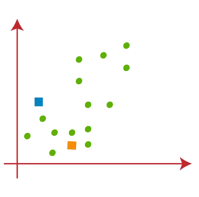

• Now we will assign each data point of the scatter plot to its closest K-point or centroid. We will compute it by applying some mathematics that we have studied to calculate the distance between two points. So, we will draw a median between both the centroids. Consider the below image:
  
  

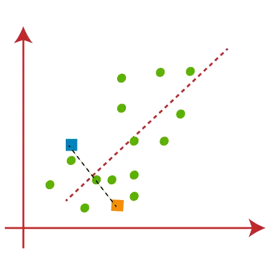
From the above image, it is clear that points left side of the line is near to the K1 or blue centroid, and points to the right of the line are close to the yellow centroid. Let's color them as blue and yellow for clear visualization.

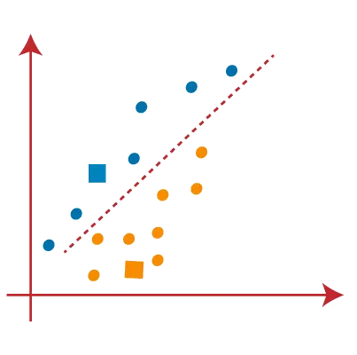
• As we need to find the closest cluster, so we will repeat the process by choosing a new centroid. To choose the new centroids, we will compute the center of gravity of these centroids, and will find new centroids as below:
  

• Next, we will reassign each datapoint to the new centroid. For this, we will repeat the same process of finding a median line. The median will be like below image:
  

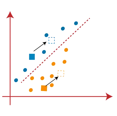
From the above image, we can see, one yellow point is on the left side of the line, and two blue points are right to the line. So, these three points will be assigned to new centroids.

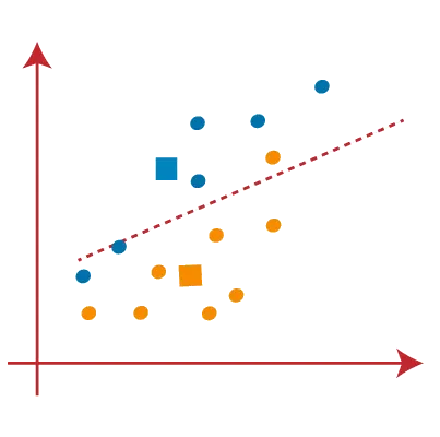
As reassignment has taken place, so we will again go to the step-4, which is finding new centroids or K-points.

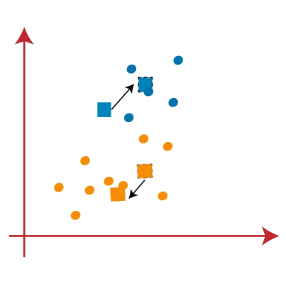
• We will repeat the process by finding the center of gravity of centroids, so the new centroids will be as shown in the below image:
  
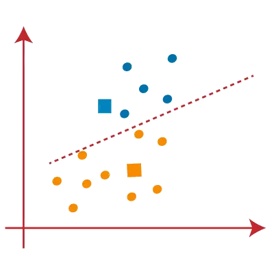
• As we got the new centroids so again will draw the median line and reassign the data points. So, the image will be:
  
  
• We can see in the above image; there are no dissimilar data points on either side of the line, which means our model is formed. Consider the below image:
  

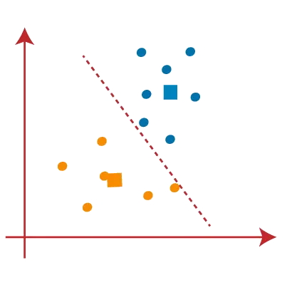
As our model is ready, so we can now remove the assumed centroids, and the two final clusters will be as shown in the below image:

How to choose the value of 'K number of Clusters' in K-Means clustering algorithm?

The performance of the K-means clustering algorithm depends upon highly efficient clusters that it forms. But choosing the optimal number of clusters is a big task. There are some different ways to find the optimal number of clusters, but here we are discussing the most appropriate method to find the number of clusters or value of K. The method is given below:

Elbow Method:

The Elbow method is one of the most popular ways to find the optimal number of clusters. This method uses the concept of WCSS value. WCSS stands for Within Cluster Sum of Squares, which defines the total variations within a cluster. The formula to calculate the value of WCSS (for 3 clusters) is given below:

WCSS=∑Pi in cluster 1distance (PiC1)2+∑Pi in cluster 2distance (PiC2)2+∑Pi in cluster 3distance (PiC3)2

In the above formula of WCSS,

∑Pi in Cluster1 distance (Pi C1)2: It is the sum of the square of the distances between each data point and its centroid within a cluster1 and the same for the other two terms.

To measure the distance between data points and centroid, we can use any method such as Euclidean distance or Manhattan distance.

To find the optimal value of clusters, the elbow method follows the below steps:-

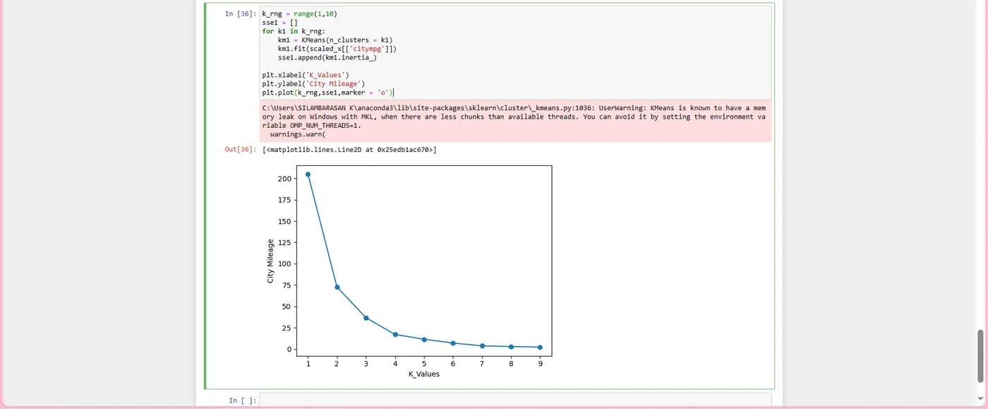
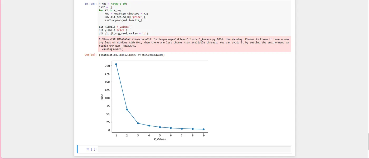
• It executes the K-means clustering on a given dataset for different K values (ranges from 1-10).
• For each value of K, calculate the WCSS value.
• Plots a curve between calculated WCSS values and the number of clusters K.
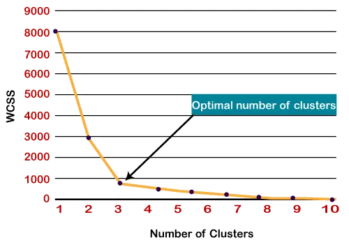
• The sharp point of bend or a point of the plot looks like an arm, then that point is considered as the best value of K.

Since the graph shows the sharp bend, which looks like an elbow, hence it is known as the elbow method. The graph for the elbow method looks like the below image:

Pros and Cons of K-Means Clustering:-

Pros:

1. Simple: It is easy to implement k-means and identify unknown groups of data from complex data sets. The results are presented in an easy and simple manner.

2. Flexible: K-means algorithm can easily adjust to the changes. If there are any problems, adjusting the cluster segment will allow changes to easily occur on the algorithm.

3. Suitable in a large dataset: K-means is suitable for a large number of datasets and it’s computed much faster than the smaller dataset. It can also produce higher clusters.

4. Efficient: The algorithm used is good at segmenting the large data set. Its efficiency depends on the shape of the clusters. K-means work well in hyper-spherical clusters.

5. Time complexity: K-means segmentation is linear in the number of data objects thus increasing execution time. It doesn’t take more time in classifying similar characteristics in data like hierarchical algorithms.

6. Tight clusters: Compared to hierarchical algorithms, k-means produce tighter clusters especially with globular clusters.

7. Easy to interpret: The results are easy to interpret. It generates cluster descriptions in a form minimized to ease understanding of the data.

8. Computation cost: Compared to using other clustering methods, a k-means clustering technique is fast and efficient in terms of its computational cost O(K*n*d).

9. Accuracy: K-means analysis improves clustering accuracy and ensures information about a particular problem domain is available. Modification of the k-means algorithm based on this information improves the accuracy of the clusters.

10. Spherical clusters: This mode of clustering works great when dealing with spherical clusters. It operates with an assumption of joint distributions of features since each cluster is spherical. All the clusters features or characters have equal variance and each is independent of each other.

Cons:

1. No-optimal set of clusters: K-means doesn’t allow development of an optimal set of clusters and for effective results, you should decide on the clusters before.

2. Lacks consistency: K-means clustering gives varying results on different runs of an algorithm. A random choice of cluster patterns yields different clustering results resulting in inconsistency.

3. Uniform effect: It produces cluster with uniform size even when the input data has different sizes.

4. Order of values: The way in which data is ordered in building the algorithm affects the final results of the data set.

5. Sensitivity to scale: Changing or rescaling the dataset either through normalization or standardization will completely change the final results.

6. Crash computer: When dealing with a large dataset, conducting a dendrogram technique will crash the computer due to a lot of computational load and Ram limits.

7. Handle numerical data: K-means algorithm can be performed in numerical data only.

8. Operates in assumption: K-means clustering technique assumes that we deal with spherical clusters and each cluster has equal numbers for observations. The spherical assumptions have to be satisfied. The algorithm can’t work with clusters of unusual size.

9. Specify K-values: For K-means clustering to be effective, you have to specify the number of clusters (K) at the beginning of the algorithm.

10. Prediction issues: It is difficult to predict the k-values or the number of clusters. It is also difficult to compare the quality of the produced clusters.

Implementing the K-Means Clustering Algorithm for 'Car Dataset':

This data set consists of three types of entities:
(a) the specification of an auto in terms of various characteristics,
(b) its assigned insurance risk rating,
(c) its normalized losses in use as compared to other cars. The second rating corresponds to the degree to which the auto is more risky than its price indicates. Cars are initially assigned a risk factor symbol associated with its price. Then, if it is more risky (or less), this symbol is adjusted by moving it up (or down) the scale. Actuaries call this process "symbolling". A value of +3 indicates that the auto is risky, -3 that it is probably pretty safe. The third factor is the relative average loss payment per insured vehicle year. This value is normalized for all autos within a particular size classification (two-door small, station wagons, sports/specialty, etc.…), and represents the average loss per car per year.

Note: Several of the attributes in the database could be used as a "class" attribute.

Number of Instances: 205

Number of Attributes: 29 total
-- 18 continuous
-- 1 integer
-- 10 nominal.

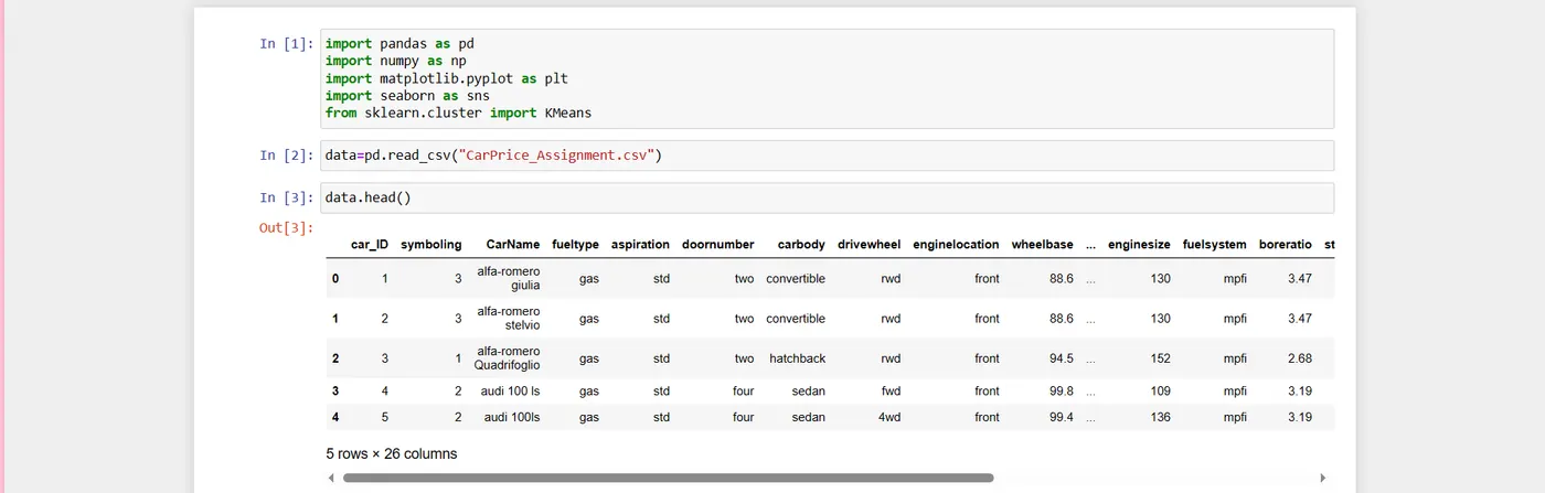
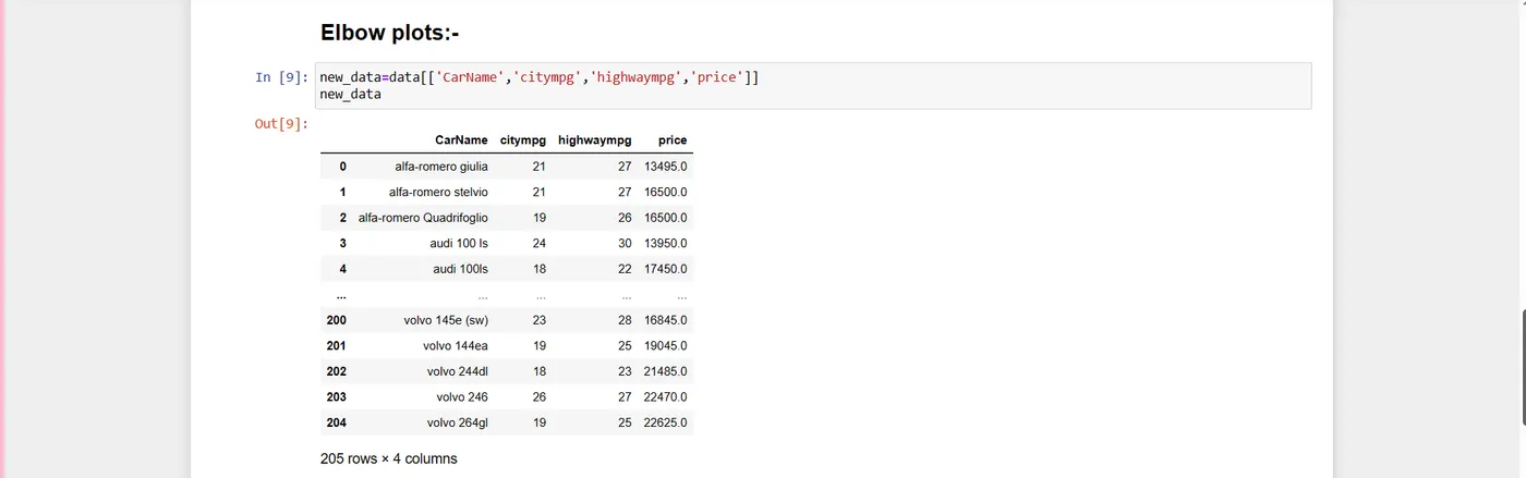
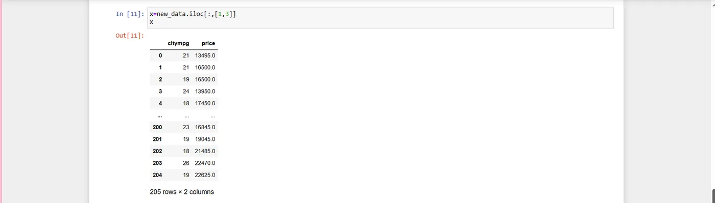
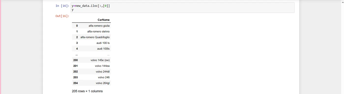
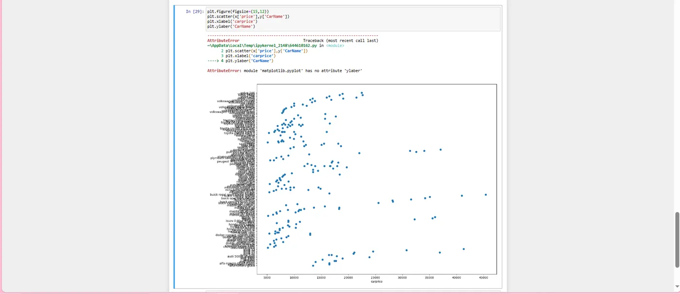
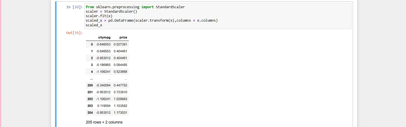
• Importing the 'Car' dataset.

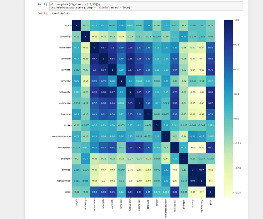
• Creating a heatmap of the correlation of all the attributes.

Implementing Hierarchical Clustering to the 'Car' Dataset:

The Steps we are going to follow to perform the algorithm are:

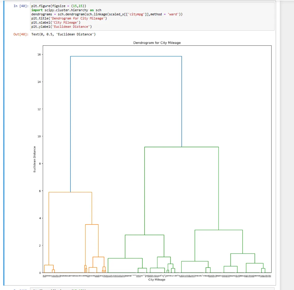
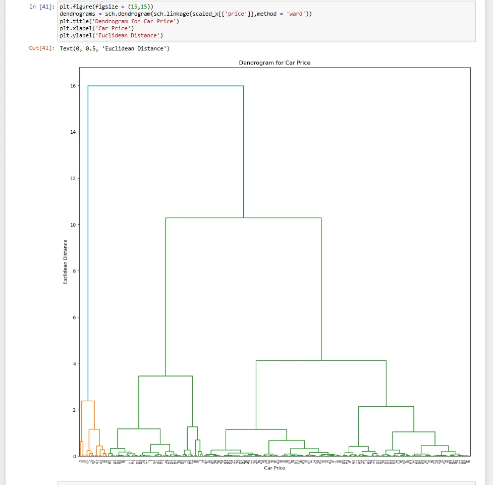
• Creating dendrograms for both the attributes,
• Implementing the Agglomerative Clustering method.
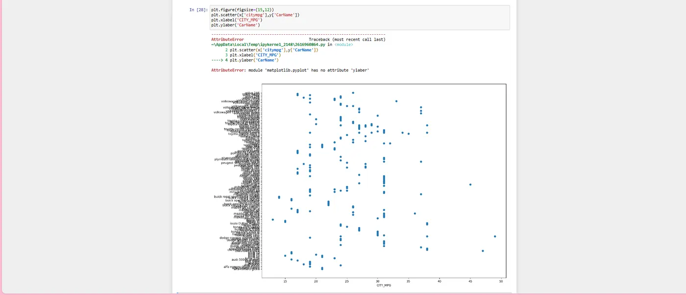
• Making Scatter plots for both attributes.