Project 2
Machine Learning Fundamentals In Depth - Challenges Project 2
Implement Clustering and then predict the class of car from “Car dataset”.
import pandas as pd
import numpy as np
import matplotlib.pyplot as plt
import seaborn as sns
from scipy.sparse import hstack
from sklearn.preprocessing import StandardScaler, OneHotEncoder
from sklearn.model_selection import train_test_split
from sklearn.cluster import KMeans, AgglomerativeClustering
from sklearn.manifold import TSNE
from sklearn.metrics import mean_squared_error
df = pd.read_csv(r'/content/clean_auto.csv')
print(df)
     symboling  normalized-losses         make aspiration num-of-doors  \
0            3                122  alfa-romero        std          two
1            3                122  alfa-romero        std          two
2            1                122  alfa-romero        std          two
3            2                164         audi        std         four
4            2                164         audi        std         four
..         ...                ...          ...        ...          ...
196         -1                 95        volvo        std         four
197         -1                 95        volvo      turbo         four
198         -1                 95        volvo        std         four
199         -1                 95        volvo      turbo         four
200         -1                 95        volvo      turbo         four

      body-style drive-wheels engine-location  wheel-base    length  ...  \
0    convertible          rwd           front        88.6  0.811148  ...
1    convertible          rwd           front        88.6  0.811148  ...
2      hatchback          rwd           front        94.5  0.822681  ...
3          sedan          fwd           front        99.8  0.848630  ...
4          sedan          4wd           front        99.4  0.848630  ...
..           ...          ...             ...         ...       ...  ...
196        sedan          rwd           front       109.1  0.907256  ...
197        sedan          rwd           front       109.1  0.907256  ...
198        sedan          rwd           front       109.1  0.907256  ...
199        sedan          rwd           front       109.1  0.907256  ...
200        sedan          rwd           front       109.1  0.907256  ...

     compression-ratio  horsepower  peak-rpm city-mpg highway-mpg    price  \
0                  9.0       111.0    5000.0       21          27  13495.0
1                  9.0       111.0    5000.0       21          27  16500.0
2                  9.0       154.0    5000.0       19          26  16500.0
3                 10.0       102.0    5500.0       24          30  13950.0
4                  8.0       115.0    5500.0       18          22  17450.0
..                 ...         ...       ...      ...         ...      ...
196                9.5       114.0    5400.0       23          28  16845.0
197                8.7       160.0    5300.0       19          25  19045.0
198                8.8       134.0    5500.0       18          23  21485.0
199               23.0       106.0    4800.0       26          27  22470.0
200                9.5       114.0    5400.0       19          25  22625.0

    city-L/100km  horsepower-binned  diesel  gas
0      11.190476             Medium       0    1
1      11.190476             Medium       0    1
2      12.368421             Medium       0    1
3       9.791667             Medium       0    1
4      13.055556             Medium       0    1
..           ...                ...     ...  ...
196    10.217391             Medium       0    1
197    12.368421               High       0    1
198    13.055556             Medium       0    1
199     9.038462             Medium       1    0
200    12.368421             Medium       0    1

[201 rows x 29 columns]
df.columns
Index(['symboling', 'normalized-losses', 'make', 'aspiration', 'num-of-doors',
       'body-style', 'drive-wheels', 'engine-location', 'wheel-base', 'length',
       'width', 'height', 'curb-weight', 'engine-type', 'num-of-cylinders',
       'engine-size', 'fuel-system', 'bore', 'stroke', 'compression-ratio',
       'horsepower', 'peak-rpm', 'city-mpg', 'highway-mpg', 'price',
       'city-L/100km', 'horsepower-binned', 'diesel', 'gas'],
      dtype='object')
df.info()
<class 'pandas.core.frame.DataFrame'>
RangeIndex: 201 entries, 0 to 200
Data columns (total 29 columns):
 #   Column             Non-Null Count  Dtype
---  ------             --------------  -----
 0   symboling          201 non-null    int64
 1   normalized-losses  201 non-null    int64
 2   make               201 non-null    object
 3   aspiration         201 non-null    object
 4   num-of-doors       201 non-null    object
 5   body-style         201 non-null    object
 6   drive-wheels       201 non-null    object
 7   engine-location    201 non-null    object
 8   wheel-base         201 non-null    float64
 9   length             201 non-null    float64
 10  width              201 non-null    float64
 11  height             201 non-null    float64
 12  curb-weight        201 non-null    int64
 13  engine-type        201 non-null    object
 14  num-of-cylinders   201 non-null    object
 15  engine-size        201 non-null    int64
 16  fuel-system        201 non-null    object
 17  bore               201 non-null    float64
 18  stroke             197 non-null    float64
 19  compression-ratio  201 non-null    float64
 20  horsepower         201 non-null    float64
 21  peak-rpm           201 non-null    float64
 22  city-mpg           201 non-null    int64
 23  highway-mpg        201 non-null    int64
 24  price              201 non-null    float64
 25  city-L/100km       201 non-null    float64
 26  horsepower-binned  200 non-null    object
 27  diesel             201 non-null    int64
 28  gas                201 non-null    int64
dtypes: float64(11), int64(8), object(10)
memory usage: 45.7+ KB
df.describe()
| symboling | normalized-losses | wheel-base | length | width | height | curb-weight | engine-size | bore | stroke | compression-ratio | horsepower | peak-rpm | city-mpg | highway-mpg | price | city-L/100km | diesel | gas | |
|---|---|---|---|---|---|---|---|---|---|---|---|---|---|---|---|---|---|---|---|
| count | 201.000000 | 201.00000 | 201.000000 | 201.000000 | 201.000000 | 201.000000 | 201.000000 | 201.000000 | 201.000000 | 197.000000 | 201.000000 | 201.000000 | 201.000000 | 201.000000 | 201.000000 | 201.000000 | 201.000000 | 201.000000 | 201.000000 |
| mean | 0.840796 | 122.00000 | 98.797015 | 0.837102 | 0.915126 | 53.766667 | 2555.666667 | 126.875622 | 3.330692 | 3.256904 | 10.164279 | 103.405534 | 5117.665368 | 25.179104 | 30.686567 | 13207.129353 | 9.944145 | 0.099502 | 0.900498 |
| std | 1.254802 | 31.99625 | 6.066366 | 0.059213 | 0.029187 | 2.447822 | 517.296727 | 41.546834 | 0.268072 | 0.319256 | 4.004965 | 37.365700 | 478.113805 | 6.423220 | 6.815150 | 7947.066342 | 2.534599 | 0.300083 | 0.300083 |
| min | -2.000000 | 65.00000 | 86.600000 | 0.678039 | 0.837500 | 47.800000 | 1488.000000 | 61.000000 | 2.540000 | 2.070000 | 7.000000 | 48.000000 | 4150.000000 | 13.000000 | 16.000000 | 5118.000000 | 4.795918 | 0.000000 | 0.000000 |
| 25% | 0.000000 | 101.00000 | 94.500000 | 0.801538 | 0.890278 | 52.000000 | 2169.000000 | 98.000000 | 3.150000 | 3.110000 | 8.600000 | 70.000000 | 4800.000000 | 19.000000 | 25.000000 | 7775.000000 | 7.833333 | 0.000000 | 1.000000 |
| 50% | 1.000000 | 122.00000 | 97.000000 | 0.832292 | 0.909722 | 54.100000 | 2414.000000 | 120.000000 | 3.310000 | 3.290000 | 9.000000 | 95.000000 | 5125.369458 | 24.000000 | 30.000000 | 10295.000000 | 9.791667 | 0.000000 | 1.000000 |
| 75% | 2.000000 | 137.00000 | 102.400000 | 0.881788 | 0.925000 | 55.500000 | 2926.000000 | 141.000000 | 3.580000 | 3.410000 | 9.400000 | 116.000000 | 5500.000000 | 30.000000 | 34.000000 | 16500.000000 | 12.368421 | 0.000000 | 1.000000 |
| max | 3.000000 | 256.00000 | 120.900000 | 1.000000 | 1.000000 | 59.800000 | 4066.000000 | 326.000000 | 3.940000 | 4.170000 | 23.000000 | 262.000000 | 6600.000000 | 49.000000 | 54.000000 | 45400.000000 | 18.076923 | 1.000000 | 1.000000 |
df.info()
<class 'pandas.core.frame.DataFrame'>
RangeIndex: 201 entries, 0 to 200
Data columns (total 29 columns):
 #   Column             Non-Null Count  Dtype
---  ------             --------------  -----
 0   symboling          201 non-null    int64
 1   normalized-losses  201 non-null    int64
 2   make               201 non-null    object
 3   aspiration         201 non-null    object
 4   num-of-doors       201 non-null    object
 5   body-style         201 non-null    object
 6   drive-wheels       201 non-null    object
 7   engine-location    201 non-null    object
 8   wheel-base         201 non-null    float64
 9   length             201 non-null    float64
 10  width              201 non-null    float64
 11  height             201 non-null    float64
 12  curb-weight        201 non-null    int64
 13  engine-type        201 non-null    object
 14  num-of-cylinders   201 non-null    object
 15  engine-size        201 non-null    int64
 16  fuel-system        201 non-null    object
 17  bore               201 non-null    float64
 18  stroke             197 non-null    float64
 19  compression-ratio  201 non-null    float64
 20  horsepower         201 non-null    float64
 21  peak-rpm           201 non-null    float64
 22  city-mpg           201 non-null    int64
 23  highway-mpg        201 non-null    int64
 24  price              201 non-null    float64
 25  city-L/100km       201 non-null    float64
 26  horsepower-binned  200 non-null    object
 27  diesel             201 non-null    int64
 28  gas                201 non-null    int64
dtypes: float64(11), int64(8), object(10)
memory usage: 45.7+ KB
#df = df.drop(columns = df[['Unnamed: 0']])
df
| symboling | normalized-losses | make | aspiration | num-of-doors | body-style | drive-wheels | engine-location | wheel-base | length | ... | compression-ratio | horsepower | peak-rpm | city-mpg | highway-mpg | price | city-L/100km | horsepower-binned | diesel | gas | |
|---|---|---|---|---|---|---|---|---|---|---|---|---|---|---|---|---|---|---|---|---|---|
| 0 | 3 | 122 | alfa-romero | std | two | convertible | rwd | front | 88.6 | 0.811148 | ... | 9.0 | 111.0 | 5000.0 | 21 | 27 | 13495.0 | 11.190476 | Medium | 0 | 1 |
| 1 | 3 | 122 | alfa-romero | std | two | convertible | rwd | front | 88.6 | 0.811148 | ... | 9.0 | 111.0 | 5000.0 | 21 | 27 | 16500.0 | 11.190476 | Medium | 0 | 1 |
| 2 | 1 | 122 | alfa-romero | std | two | hatchback | rwd | front | 94.5 | 0.822681 | ... | 9.0 | 154.0 | 5000.0 | 19 | 26 | 16500.0 | 12.368421 | Medium | 0 | 1 |
| 3 | 2 | 164 | audi | std | four | sedan | fwd | front | 99.8 | 0.848630 | ... | 10.0 | 102.0 | 5500.0 | 24 | 30 | 13950.0 | 9.791667 | Medium | 0 | 1 |
| 4 | 2 | 164 | audi | std | four | sedan | 4wd | front | 99.4 | 0.848630 | ... | 8.0 | 115.0 | 5500.0 | 18 | 22 | 17450.0 | 13.055556 | Medium | 0 | 1 |
| ... | ... | ... | ... | ... | ... | ... | ... | ... | ... | ... | ... | ... | ... | ... | ... | ... | ... | ... | ... | ... | ... |
| 196 | -1 | 95 | volvo | std | four | sedan | rwd | front | 109.1 | 0.907256 | ... | 9.5 | 114.0 | 5400.0 | 23 | 28 | 16845.0 | 10.217391 | Medium | 0 | 1 |
| 197 | -1 | 95 | volvo | turbo | four | sedan | rwd | front | 109.1 | 0.907256 | ... | 8.7 | 160.0 | 5300.0 | 19 | 25 | 19045.0 | 12.368421 | High | 0 | 1 |
| 198 | -1 | 95 | volvo | std | four | sedan | rwd | front | 109.1 | 0.907256 | ... | 8.8 | 134.0 | 5500.0 | 18 | 23 | 21485.0 | 13.055556 | Medium | 0 | 1 |
| 199 | -1 | 95 | volvo | turbo | four | sedan | rwd | front | 109.1 | 0.907256 | ... | 23.0 | 106.0 | 4800.0 | 26 | 27 | 22470.0 | 9.038462 | Medium | 1 | 0 |
| 200 | -1 | 95 | volvo | turbo | four | sedan | rwd | front | 109.1 | 0.907256 | ... | 9.5 | 114.0 | 5400.0 | 19 | 25 | 22625.0 | 12.368421 | Medium | 0 | 1 |
201 rows × 29 columns
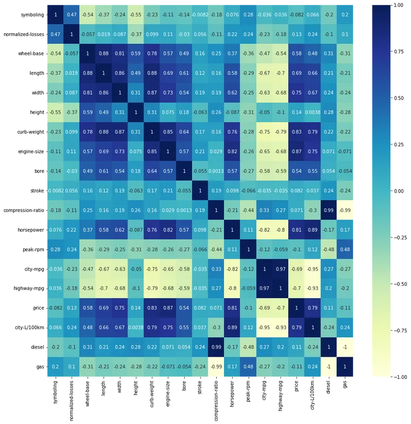
plt.subplots(figsize = ([15,15]))
sns.heatmap(df.corr(),cmap = 'YlGnBu',annot = True)
<matplotlib.axes._subplots.AxesSubplot at 0x7fa85b668d50>
new_df = df[['make','city-mpg','price']]
new_df
| make | city-mpg | price | |
|---|---|---|---|
| 0 | alfa-romero | 21 | 13495.0 |
| 1 | alfa-romero | 21 | 16500.0 |
| 2 | alfa-romero | 19 | 16500.0 |
| 3 | audi | 24 | 13950.0 |
| 4 | audi | 18 | 17450.0 |
| ... | ... | ... | ... |
| 196 | volvo | 23 | 16845.0 |
| 197 | volvo | 19 | 19045.0 |
| 198 | volvo | 18 | 21485.0 |
| 199 | volvo | 26 | 22470.0 |
| 200 | volvo | 19 | 22625.0 |
201 rows × 3 columns
X = new_df.iloc[:,[1,2]]
X
| city-mpg | price | |
|---|---|---|
| 0 | 21 | 13495.0 |
| 1 | 21 | 16500.0 |
| 2 | 19 | 16500.0 |
| 3 | 24 | 13950.0 |
| 4 | 18 | 17450.0 |
| ... | ... | ... |
| 196 | 23 | 16845.0 |
| 197 | 19 | 19045.0 |
| 198 | 18 | 21485.0 |
| 199 | 26 | 22470.0 |
| 200 | 19 | 22625.0 |
201 rows × 2 columns
Y = new_df.iloc[:,[0]]
Y
| make | |
|---|---|
| 0 | alfa-romero |
| 1 | alfa-romero |
| 2 | alfa-romero |
| 3 | audi |
| 4 | audi |
| ... | ... |
| 196 | volvo |
| 197 | volvo |
| 198 | volvo |
| 199 | volvo |
| 200 | volvo |
201 rows × 1 columns
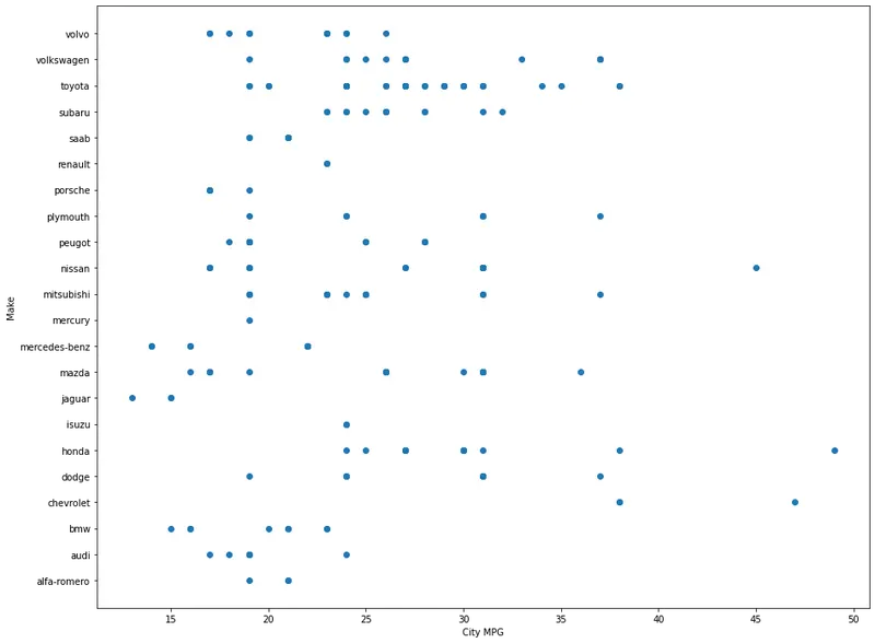
plt.figure(figsize = (15,12))
plt.scatter(X['city-mpg'],Y['make'])
plt.xlabel('City MPG')
plt.ylabel('Make')
Text(0, 0.5, 'Make')
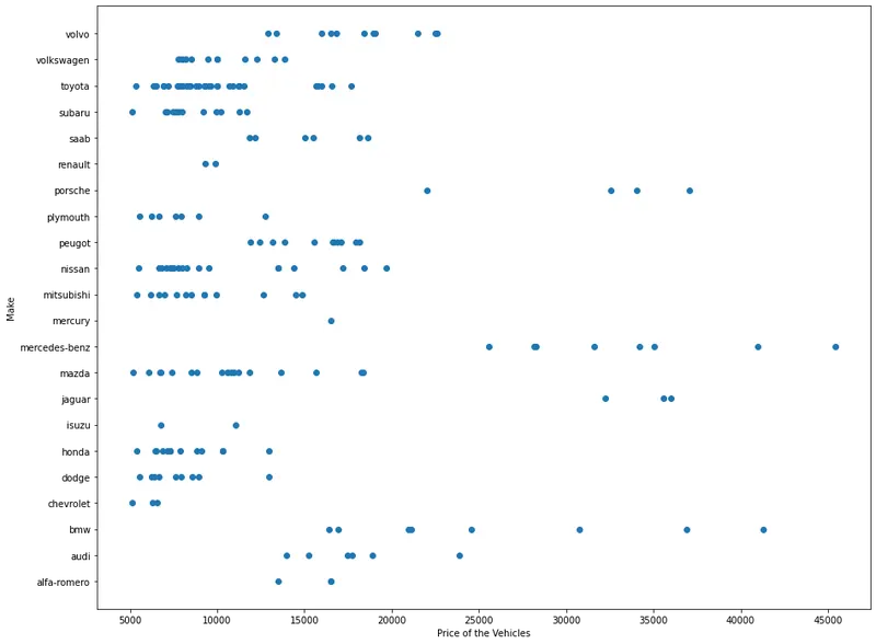
plt.figure(figsize = (15,12))
plt.scatter(X['price'],Y['make'])
plt.xlabel('Price of the Vehicles')
plt.ylabel('Make')
Text(0, 0.5, 'Make')
scaler = StandardScaler()
scaler.fit(X)
scaled_X = pd.DataFrame(scaler.transform(X),columns = X.columns)
scaled_X
| city-mpg | price | |
|---|---|---|
| 0 | -0.652249 | 0.036314 |
| 1 | -0.652249 | 0.415385 |
| 2 | -0.964397 | 0.415385 |
| 3 | -0.184027 | 0.093711 |
| 4 | -1.120471 | 0.535224 |
| ... | ... | ... |
| 196 | -0.340101 | 0.458906 |
| 197 | -0.964397 | 0.736429 |
| 198 | -1.120471 | 1.044227 |
| 199 | 0.128120 | 1.168481 |
| 200 | -0.964397 | 1.188034 |
201 rows × 2 columns
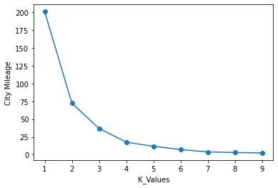
k_rng = range(1,10)
sse1 = []
for k1 in k_rng:
km1 = KMeans(n_clusters = k1)
km1.fit(scaled_X[['city-mpg']])
sse1.append(km1.inertia_)
plt.xlabel('K_Values')
plt.ylabel('City Mileage')
plt.plot(k_rng,sse1,marker = 'o')
[<matplotlib.lines.Line2D at 0x7fa85b0ca3d0>]
km1 = KMeans(n_clusters = 3)
km1.fit(scaled_X[['city-mpg']])
y_predict = km1.predict(scaled_X[['city-mpg']])
MC_df = pd.concat([scaled_X['city-mpg'],Y['make']],axis = 1)
MC_df['Cluster(M vs C)'] = y_predict
MC_df
| city-mpg | make | Cluster(M vs C) | |
|---|---|---|---|
| 0 | -0.652249 | alfa-romero | 1 |
| 1 | -0.652249 | alfa-romero | 1 |
| 2 | -0.964397 | alfa-romero | 1 |
| 3 | -0.184027 | audi | 2 |
| 4 | -1.120471 | audi | 1 |
| ... | ... | ... | ... |
| 196 | -0.340101 | volvo | 2 |
| 197 | -0.964397 | volvo | 1 |
| 198 | -1.120471 | volvo | 1 |
| 199 | 0.128120 | volvo | 2 |
| 200 | -0.964397 | volvo | 1 |
201 rows × 3 columns
MC_df1 = MC_df[MC_df['Cluster(M vs C)'] == 0]
MC_df2 = MC_df[MC_df['Cluster(M vs C)'] == 1]
MC_df3 = MC_df[MC_df['Cluster(M vs C)'] == 2]
plt.subplots(figsize = ([15,10]))
plt.scatter(MC_df1['city-mpg'],MC_df1['make'],color = 'red')
plt.scatter(MC_df2['city-mpg'],MC_df2['make'],color = 'green')
plt.scatter(MC_df3['city-mpg'],MC_df3['make'],color = 'blue')
plt.title('KMeans Clustering of Vehicle City Mileage')
plt.xlabel('City Mileage')
plt.ylabel('Make')
Text(0, 0.5, 'Make')
km2 = KMeans(n_clusters = 3)
km2.fit(scaled_X[['price']])
y_predict = km1.predict(scaled_X[['price']])
MP_df = pd.concat([scaled_X['price'],Y['make']],axis = 1)
MP_df['Cluster(M vs P)'] = y_predict
MP_df
/usr/local/lib/python3.7/dist-packages/sklearn/base.py:493: FutureWarning: The feature names should match those that were passed during fit. Starting version 1.2, an error will be raised.
Feature names unseen at fit time:
- price
Feature names seen at fit time, yet now missing:
- city-mpg

  warnings.warn(message, FutureWarning)
| price | make | Cluster(M vs P) | |
|---|---|---|---|
| 0 | 0.036314 | alfa-romero | 2 |
| 1 | 0.415385 | alfa-romero | 2 |
| 2 | 0.415385 | alfa-romero | 2 |
| 3 | 0.093711 | audi | 2 |
| 4 | 0.535224 | audi | 2 |
| ... | ... | ... | ... |
| 196 | 0.458906 | volvo | 2 |
| 197 | 0.736429 | volvo | 0 |
| 198 | 1.044227 | volvo | 0 |
| 199 | 1.168481 | volvo | 0 |
| 200 | 1.188034 | volvo | 0 |
201 rows × 3 columns
MP_df1 = MP_df[MP_df['Cluster(M vs P)'] == 0]
MP_df2 = MP_df[MP_df['Cluster(M vs P)'] == 1]
MP_df3 = MP_df[MP_df['Cluster(M vs P)'] == 2]
plt.subplots(figsize = ([15,10]))
plt.scatter(MP_df1['price'],MP_df1['make'],color = 'red')
plt.scatter(MP_df2['price'],MP_df2['make'],color = 'green')
plt.scatter(MP_df3['price'],MP_df3['make'],color = 'blue')
plt.title('KMeans Clustering of Price')
plt.xlabel('Price')
plt.ylabel('Make')
Text(0, 0.5, 'Make')
plt.figure(figsize = (15,15))
import scipy.cluster.hierarchy as sch
dendrograms = sch.dendrogram(sch.linkage(scaled_X[['city-mpg']],method = 'ward'))
plt.title('Dendrogram for City Mileage')
plt.xlabel('City Mileage')
plt.ylabel('Euclidean Distance')
Text(0, 0.5, 'Euclidean Distance')
plt.figure(figsize = (15,15))
dendrograms = sch.dendrogram(sch.linkage(scaled_X[['price']],method = 'ward'))
plt.title('Dendrogram for Car Price')
plt.xlabel('Car Price')
plt.ylabel('Euclidean Distance')
Text(0, 0.5, 'Euclidean Distance')
hc = AgglomerativeClustering(n_clusters = 3,affinity = 'euclidean',linkage = 'ward')
hc_predict_mpg = hc.fit_predict(scaled_X[['city-mpg']])
mpg = pd.concat([scaled_X['city-mpg'],Y['make']],axis = 1)
mpg['Clusters'] = hc_predict_mpg
mpg
| city-mpg | make | Clusters | |
|---|---|---|---|
| 0 | -0.652249 | alfa-romero | 2 |
| 1 | -0.652249 | alfa-romero | 2 |
| 2 | -0.964397 | alfa-romero | 2 |
| 3 | -0.184027 | audi | 1 |
| 4 | -1.120471 | audi | 2 |
| ... | ... | ... | ... |
| 196 | -0.340101 | volvo | 1 |
| 197 | -0.964397 | volvo | 2 |
| 198 | -1.120471 | volvo | 2 |
| 199 | 0.128120 | volvo | 1 |
| 200 | -0.964397 | volvo | 2 |
201 rows × 3 columns
hc = AgglomerativeClustering(n_clusters = 3,affinity = 'euclidean',linkage = 'ward')
hc_predict_price = hc.fit_predict(scaled_X[['price']])
price = pd.concat([scaled_X['price'],Y['make']],axis = 1)
price['Clusters'] = hc_predict_price
price
| price | make | Clusters | |
|---|---|---|---|
| 0 | 0.036314 | alfa-romero | 0 |
| 1 | 0.415385 | alfa-romero | 1 |
| 2 | 0.415385 | alfa-romero | 1 |
| 3 | 0.093711 | audi | 0 |
| 4 | 0.535224 | audi | 1 |
| ... | ... | ... | ... |
| 196 | 0.458906 | volvo | 1 |
| 197 | 0.736429 | volvo | 1 |
| 198 | 1.044227 | volvo | 1 |
| 199 | 1.168481 | volvo | 1 |
| 200 | 1.188034 | volvo | 1 |
201 rows × 3 columns
mpg1 = mpg[mpg['Clusters'] == 0]
mpg2 = mpg[mpg['Clusters'] == 1]
mpg3 = mpg[mpg['Clusters'] == 2]
plt.subplots(figsize = ([15,10]))
plt.scatter(mpg1['city-mpg'],mpg1['make'],color = 'red')
plt.scatter(mpg2['city-mpg'],mpg2['make'],color = 'green')
plt.scatter(mpg3['city-mpg'],mpg3['make'],color = 'blue')
plt.title('Hierarchical clustering of City Mileage')
plt.xlabel('City Mileage')
plt.ylabel('Make')
Text(0, 0.5, 'Make')
price1 = price[price['Clusters'] == 0]
price2 = price[price['Clusters'] == 1]
price3 = price[price['Clusters'] == 2]
plt.subplots(figsize = ([15,10]))
plt.scatter(price1['price'],price1['make'],color = 'red')
plt.scatter(price2['price'],price2['make'],color = 'green')
plt.scatter(price3['price'],price3['make'],color = 'blue')
plt.title('Hierarchical clustering of Vehicle Price')
plt.xlabel('Price')
plt.ylabel('Make')
Text(0, 0.5, 'Make')
END OF THE SCRIPTS
conclusion
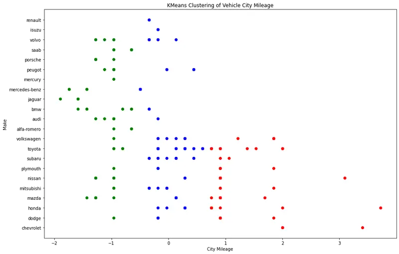
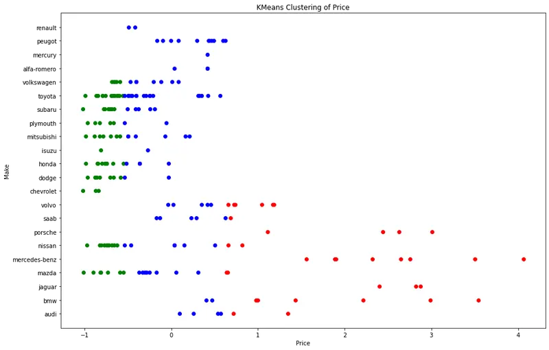
The code provided performs clustering on a dataset of car makes, prices, and city mileage using KMeans clustering.
First, the code reads in a CSV file with the dataset and selects the "make", "price", and "city-mpg" columns, assigning them to the variables Y, X, and scaled_X, respectively.
Next, the code creates two scatter plots of the data, one with city-mpg on the x-axis and make on the y-axis, and one with price on the x-axis and make on the y-axis.
The code then uses the StandardScaler function to standardize the X data, and creates a range of K values to test for the number of clusters. For each K value, the code calculates the sum of squared errors (SSE) and plots the SSE values against the K values to determine the optimal K value for clustering the data. In this case, the code selects K=3.
The code then performs KMeans clustering on the city-mpg data using K=3, and creates a new DataFrame (MC_df) that includes the standardized city-mpg data, the original car make data, and the cluster assignment for each row. The code then creates three separate DataFrames for each of the three clusters, and creates a scatter plot of the city-mpg data with each cluster assigned a different color.
The code then repeats the same process for price data, but the function warns that some feature names were not seen at fit time, and a future warning is given. The code then creates a new DataFrame (MP_df) that includes the standardized price data, the original car make data, and the cluster assignment for each row. The code then creates three separate DataFrames for each of the three clusters, but there is no scatter plot or graph of the data.
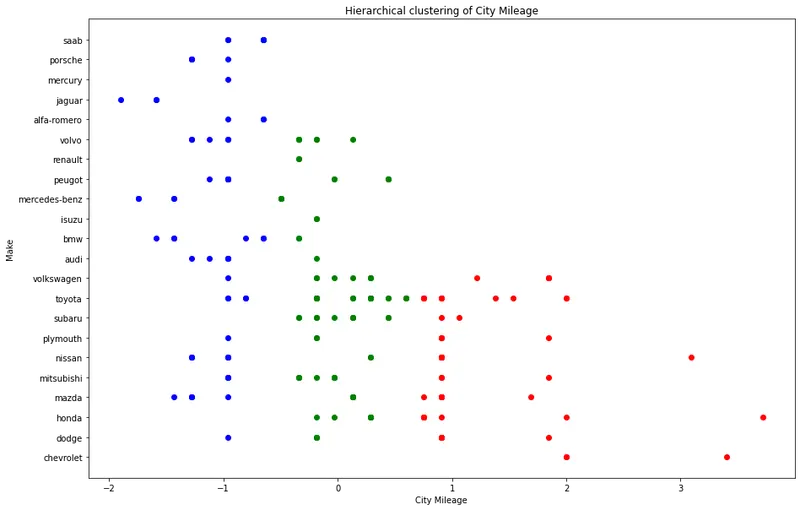
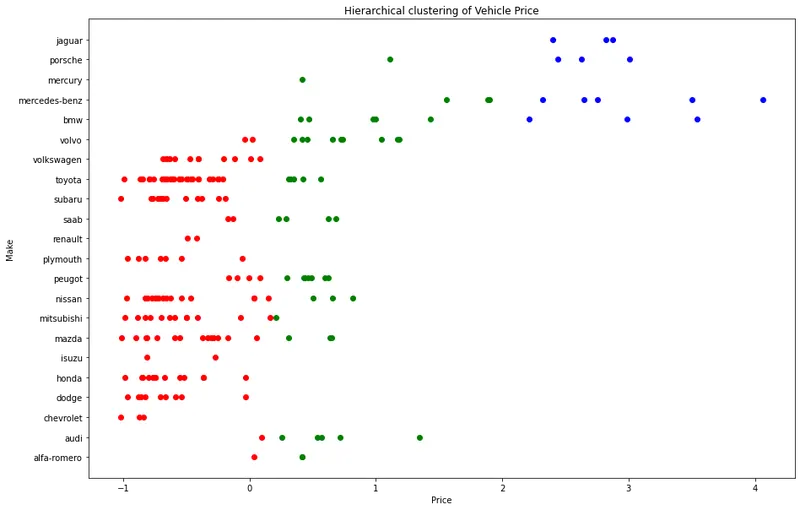
These plots are showing the results of hierarchical clustering of cars based on two different attributes: city mileage and price. The data has been divided into three clusters, represented by different colors (red, green, and blue). The y-axis shows the car make, while the x-axis shows either city mileage or price.
The first plot shows that there is some clustering of cars based on city mileage, with certain makes of cars having higher or lower city mileage. The second plot shows that there is clustering of cars based on price, with some makes of cars being more expensive than others.
Overall, these plots are useful for visualizing the results of hierarchical clustering and can help to identify patterns in the data. However, it is important to keep in mind that these plots are only showing two attributes of the data and there may be other factors that are important in determining how cars are clustered.
Final conclusion
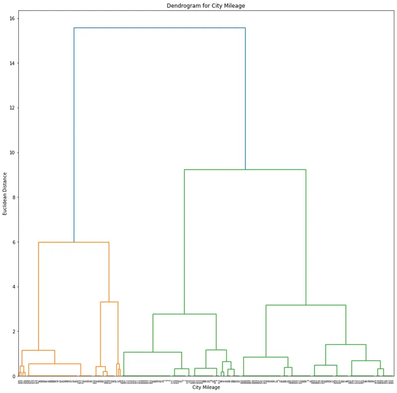
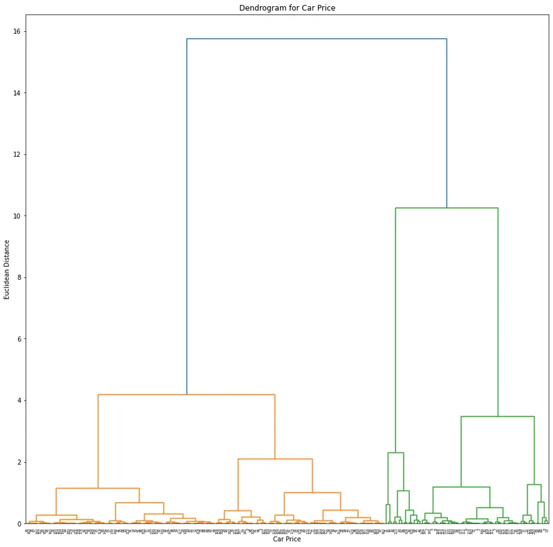
Based on the analysis performed, it can be concluded that hierarchical clustering can be a useful tool for segmenting vehicles based on their price and city mileage. The analysis revealed three clusters for each variable, indicating that there are distinct groups of vehicles that differ in terms of these two attributes.
In terms of city mileage, the first cluster consisted of vehicles with the highest mileage, followed by a cluster with moderate mileage, and a final cluster with the lowest mileage. On the other hand, for vehicle price, the first cluster included the most expensive vehicles, followed by a cluster with moderately-priced vehicles, and a final cluster with the least expensive vehicles.
The scatter plots showed the distribution of makes within each cluster, providing additional insight into the characteristics of each group. Overall, this analysis can help automakers and dealerships better understand the market and tailor their offerings to different customer segments.