Project 1 - Parsing NASA thermodynamic data

Aim:

To write a Matlab code to find the 14 coefficients of NASA thermodynamic data file and calculating the Specific heat, Enthalpy, Entropy value variations with Temperature, for all the species in data file. Also to provide 2D plots of each species and their respective molecular weights.

Procedure:

File parsing is used to read the data file provided and extract into a usable form. The code is structured to find all the 14 coefficients with temperature condition provided. After which Specific heat(Cp), Enthalpy(H), Entropy(S) are calculated using the equations provided below

`(Cp)/R=c1+c2T+c3T^2+c4T^3+c5T^4`

`H/(RT)=c1+c2T/2+(c3T^2)/3+(c4T^3)/4+(c5T^4)/5+((c6)/T)`

`S/R=c1lnT+c2T+(c3T^2)/2+(c4T^3)/3+(c5T^4)/4+c7`

T = local temperature; c1-c7 = high temperature coefficients; c8-c14 = low temperature coefficients; R = Universal gas constant = 8.314 Jmol^-1K^-1

Matlab code from lines 1 to 117:

clear all
close all
clc

f1 = fopen('THERMO.dat', 'r');
fgetl(f1);
tline = fgetl(f1);
A = strsplit(tline,' ');
Global_low_temperature = str2double(A{2});
Global_high_temperature = str2double(A{4});
Global_avg_temperature = str2double(A{3});

%Lines
for i = 3:5
    g= fgetl(f1);
end

%TEMPERATURE
for j=1:53
    species = fgetl(f1);
    t = strfind(species,'.');
    %for local temperature
    species(52-3:52+3);
    T1 = species(52-3:t(1)+3);
    T11 = str2double(T1);
    
    species(t(1)+6:62+3);
    Th1 = species(t(1)+6:t(2)+3);
    Th1_1 = str2double(Th1);
    
    species(t(2)+6:72+3);
    Tm1 = species(t(2)+6:t(3)+3);
    Tm1_1 = str2double(Tm1);
    
    species_name = species(1:6);
    
    %co-efficients for eq.1
    coeff_line_1 = fgetl(f1);
    A11 = strfind(coeff_line_1,'E');
    coeff_line_1(1:12+3);
    
    a1 = coeff_line_1(1:A11(1)+3);
    c1 = str2double(a1);
    a2 = coeff_line_1(A11(1)+4:A11(2)+3);
    c2 = str2double(a2);
    a3 = coeff_line_1(A11(2)+4:A11(3)+3);
    c3 = str2double(a3);
    a4 = coeff_line_1(A11(3)+4:A11(4)+3);
    c4 = str2double(a4);
    a5 = coeff_line_1(A11(4)+4:A11(5)+3);
    c5 = str2double(a5);
    
    %co-efficients for eq.2
    coeff_line_2 = fgetl(f1);
    A12 = strfind(coeff_line_2,'E');
    coeff_line_2(1:12+3);
    
    a6 = coeff_line_2(1:A12(1)+3);
    c6 = str2double(a6);
    a7 = coeff_line_1(A12(1)+4:A11(2)+3);
    c7 = str2double(a7);
    a8 = coeff_line_1(A12(2)+4:A11(3)+3);
    c8 = str2double(a8);
    a9 = coeff_line_1(A12(3)+4:A11(4)+3);
    c9 = str2double(a9);
    a10 = coeff_line_1(A12(4)+4:A11(5)+3);
    c10 = str2double(a10);
    
    %co-efficients for eq.3
    coeff_line_3 = fgetl(f1);
    A13 = strfind(coeff_line_3,'E');
    coeff_line_3(1:12+3);
    
    a11 = coeff_line_2(1:A13(1)+3);
    c11 = str2double(a11);
    a12 = coeff_line_1(A13(1)+4:A11(2)+3);
    c12 = str2double(a12);
    a13 = coeff_line_1(A13(2)+4:A11(3)+3);
    c13 = str2double(a13);
    a14 = coeff_line_1(A13(3)+4:A11(4)+3);
    c14 = str2double(a14);
    
    T = linspace(T11,Th1_1,100);
    R = 8.314 % Universal gas constant
    [Cp,H,S] = inputs_function(T,R,Tm1_1,c1,c2,c3,c4,c5,c6,c7,c8,c9,c10,c11,c12,c13,c14);
    mkdir('C:\Users\Vamsi\Documents\Skill-lync challenges\File parsing',species_name)
    %plotting
    figure(1)
    plot(T,Cp,'Linewidth',3,'Color','b');
    xlabel('Temperature');
    ylabel('Specific Heat');
    title(species_name);
    
    figure(2)
    plot(T,H,'Linewidth',3,'color','b')
    xlabel('Temperature')
    ylabel('Enthaply')
    title(species_name)
    
    figure(3)
    plot(T,S,'Linewidth',3,'color','b')
    xlabel('Temperature')
    ylabel('Entropy')
    title(species_name)
    
    program = (['C:\Users\Vamsi\Documents\Skill-lync challenges\File parsing\',species_name]);
    cd(program)
    
    saveas(1,'Specific Heat.jpg')
    saveas(2,'Enthalpy.jpg')
    saveas(3,'Entropy.jpg')
    cd('C:\Users\Vamsi\Documents\Skill-lync challenges')
    
    molecular_weight_calculation = molecular_weight(species_name)
end

fclose(f1)

In line 5,6 of main code, we use fopen command to read the required Thermo.dat data file and fgetl is used to extract the data in it.

In line 8 to 16, Global temperature ranges are separated using strsplit command sorted using fget command with the selected column number and skipping the unrequired lines.

In line 19 to 33, for loop command is used to get temperatures and to find the coefficients respectively strfind command is used from array ‘A’ created while extracting data. As the data is in string format, str2double or str2num can be used to convert into numbers but str2double is used for better accuracy.

Inputs_function is defined to function is defined to input the equations for calculating specific heat, Cp, Enthalpy, H & Entropy, S at respective local temperatures during which higher(c1-c7) and lower(c8-c14) temperature coefficients are segmented using if else condition.

inputs_function code:

function [Cp,H,S] = inputs_function(T,R,Tm1_1,c1,c2,c3,c4,c5,c6,c7,c8,c9,c10,c11,c12,c13,c14)
 %function is defined to input the equations for calculating Cp, H& S at
 %respective local temperatures during which higher and lower temperature coefficients
 %are segmented using if else condition
for i= 1:length(T)
    %High Temperature Coefficients
    if T(i)>Tm1_1
        Cp = (c1+ c2.*T+ c3.*T.^2 + c4.*T.^3+ c5.*T.^4).*R;
        H = (c1+(c2.*T)./2+(c3.*T.^2)./3+(c4.*T.^3)./4+ (c5.*T.^4)./5+ c6./T).*T.*R;
        S = (c1.*log(T)+c2.*T+(c3.*T.^2)./2+(c4.*T.^3)./3+(c5.*T.^4)./4+c7).*R;
        %Low Temperature Coefficients
    else
        Cp = (c8+ c9.*T+ c10.*T.^2 + c11.*T.^3+ c12.*T.^4).*R;
        H = (c8+(c9.*T)./2+(c10.*T.^2)./3+(c11.*T.^3)./4+ (c12.*T.^4)./5+ c13./T).*R;
        S = (c8.*log(T)+c9.*T+(c10.*T.^2)./2+(c11.*T.^3)./3+(c12.*T.^4)./4+c14).*R;
    end
end
end

In line 35 to 81, coefficients from each column of the matrix ‘A’ are assigned to coefficient array c1 to c14 for each species using strfind command which are converted to numbers using str2double.

In line 83 &84, temperature array from global low temperature to global high temperature is created using linspace command.

In line 85, inputs_function is called for calculating specific heat Cp, enthalpy H and entropy S for each species using respective coefficients at high temperature and low temperature with reference to the mean temperature.

In line 86, mkdir command is used to create a directory based on species name for accommodating the required plots into a folder inside the chosen path within the system.

In line 88 to 104, figures 1, 2 and 3 are plotted between Cp Vs T, H Vs T, S Vs T for each species.

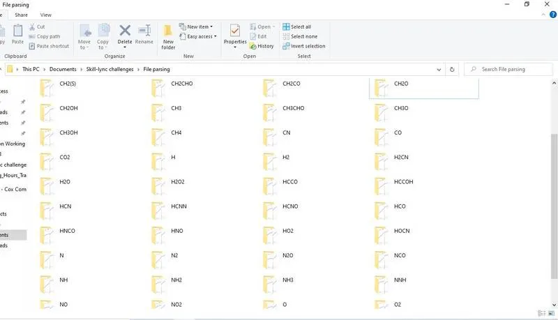
In line 106 to 112, program and saveas commands are used to store figures 1, 2 and 3 in specified species folder.

Molecular_weight function is defined to calculate the species molecular weight based on the atomic mass of each element forming species name. Two ‘for loops’ are defined to identify the element and number of counts of it in the species name using strcmp command.

molecular_weight function code:

function molecular_weight_calculation = molecular_weight(species_name)
%molecular weight calculation function by species name
species = (species_name);
elements = ['H','C','O','N','A','S'];
atomic_mass = [1.00794 12.0107 15.999 14.0067 39.948 36];
molecular_weight_calculation = 0;
for j=1:length(species)
for k=1:length(elements)
    if strcmp(species(j),elements(k))
        molecular_weight_calculation = molecular_weight_calculation+atomic_mass(k);
        a=k;
    end
end
n = str2double(species(j));
fprintf(species(j))
if  n>1
    molecular_weight_calculation = molecular_weight_calculation+atomic_mass(a)*(n-1);
end
end

In line 114, molecular weight of species is calculated by calling the molecular_weight function.

Google drive link to the saved folders:

https://drive.google.com/drive/folders/14dtqmPEaQ8I--FUG0OdtD0fmfsm6kZGI?usp=sharing

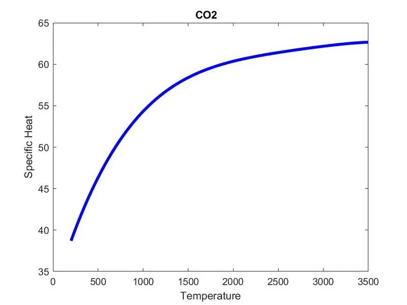
Plots for O2, N2 and CO2 are as below:

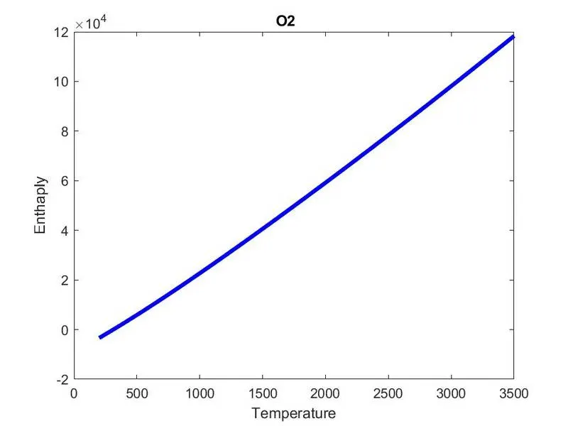
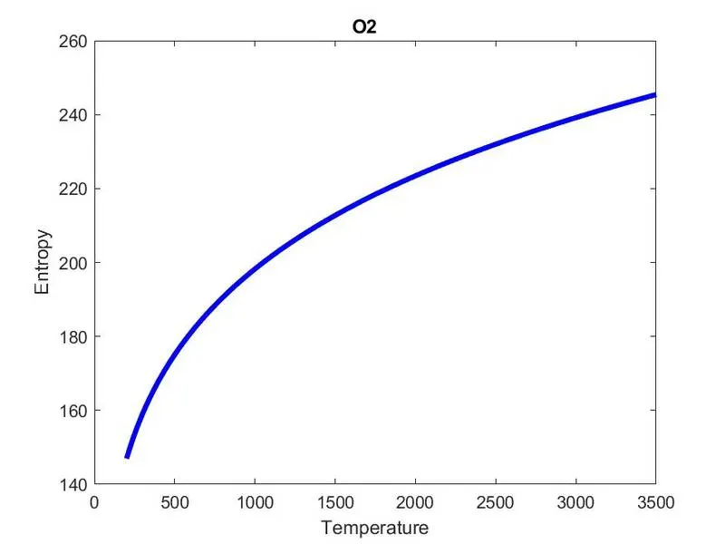
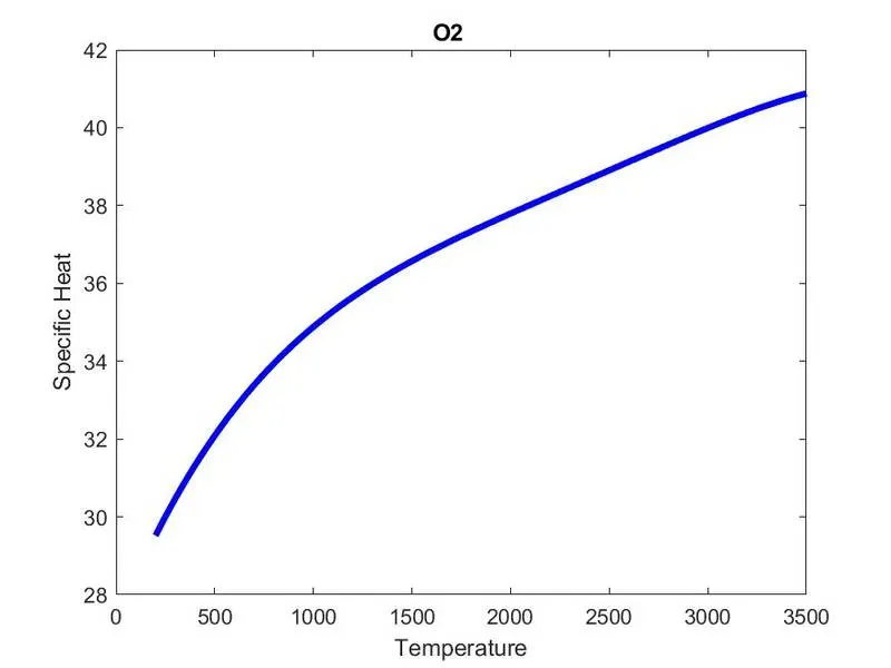
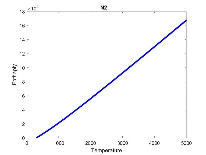
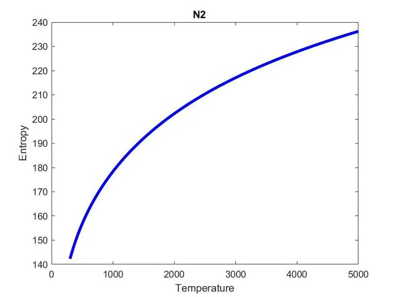
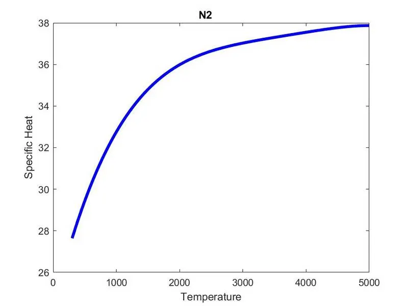
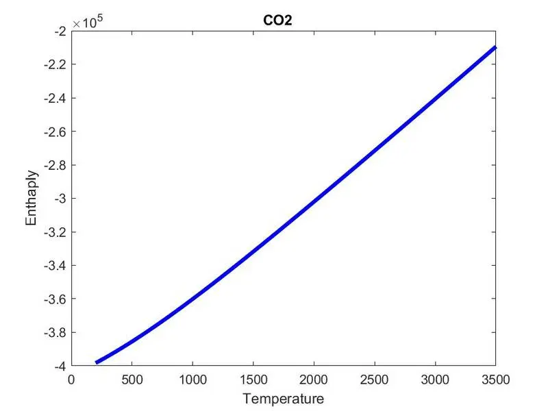
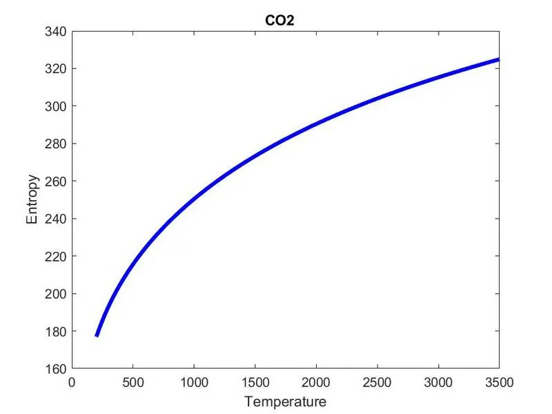
Also the screenshot of folder in which all the species plots are stored in is as below:

Conclusion:

NASA thermodynamic file has been parsed to calculate Specific heat, Enthalpy and Entropy of each species along with their molecular weight. All the plots for each species are generated and stored in separate folders automatically within the designated path as shared in google drive link.