Project 1 - Parsing NASA thermodynamic data
Aim: File parsing of NASA thermodynamic data
Objectives:
- Methodology to extract element, local temperature ranges, high and low temperature co-efficients for particular species from the dat file.
- Calculate the specific heat, enthalpy and entropy for different species.
- Plot the specific heat, enthalpy and entropy for the local temperature ranges.
- Save the plots as images in .jpg or .png format and placing them in the folder with the species name.
- Calculate the molecular weight for the particular species.
Equations used to find thermodynamic properties of different species:
Specific heat `c_p = R*(a_1 + a_2*T + a_3*T^2 + a_4*T^3 + a_5*T^4)`
Enthalpy `h = R*T*(a_1 + a_2*T /2+ a_3*T^2/3 + a_4*T^3/4 + a_5*T^4/5+a_6/T)`
Entropy `S = R*(a_1*ln(T) + a_2*T + a_3*T^2/2 + a_4*T^3/3 + a_5*T^4/4 + a_7)`
Where,
R = gas constant = 8.314 KJ/Kg-K.
T = temperature in K.
`a_1, a_2, a_3, a_4, a_5, a_6, a_7` are high temperature co-efficients.
`b_1, b_2, b_3, b_4, b_5, b_6, b_7` are low temperature co-efficients.
Project code:
clear all
close all
clc

f = fopen('THERMO.dat','r');
fgetl(f);
temp = fscanf(f,'%f',[1 3]);
fgetl(f);                           %skip the comments
fgetl(f);
fgetl(f);
fgetl(f);

%Input
elem = 'CO2'
%Data extraction
%Read low and high temperature co-efficients in form of strings
for(i = 1:53)
    element = fscanf(f,'%s',[1]);

    row = fgetl(f);
    row1 = fgetl(f);
    a = findstr(row1,'E');

        s_a1 = row1(1:a(1)+3);
        s_a2 = row1(a(1)+4:a(2)+3);
        s_a3 = row1(a(2)+4:a(3)+3);
        s_a4 = row1(a(3)+4:a(4)+3);
        s_a5 = row1(a(4)+4:a(5)+3);

    row2 = fgetl(f);
    b = findstr(row2,'E');
        s_b1 = row2(1:b(1)+3);
        s_b2 = row2(b(1)+4:b(2)+3);
        s_b3 = row2(b(2)+4:b(3)+3);
        s_b4 = row2(b(3)+4:b(4)+3);
        s_b5 = row2(b(4)+4:b(5)+3);
    row3 = fgetl(f);
    c = findstr(row3,'E');
        s_c1 = row3(1:c(1)+3);
        s_c2 = row3(c(1)+4:c(2)+3);
        s_c3 = row3(c(2)+4:c(3)+3);
        s_c4 = row3(c(3)+4:c(4)+3);

     if(size(element) == size(elem))
         if(element == elem)
         break;
         end
     end
end

%Conversion of string to number
%high temperature co-effiecients
a1 = str2num(s_a1);
a2 = str2num(s_a2);
a3 = str2num(s_a3);
a4 = str2num(s_a4);
a5 = str2num(s_a5);
a6 = str2num(s_b1);
a7 = str2num(s_b2);

%low temperature co-effiecients
b1 = str2num(s_b3);
b2 = str2num(s_b4);
b3 = str2num(s_b5);
b4 = str2num(s_c1);
b5 = str2num(s_c2);
b6 = str2num(s_c3);
b7 = str2num(s_c4);

%temperature ranges
temp_row = reverse(row)
rev_temp = temp_row(6:32)
temp = reverse(rev_temp)
s_low_temp = temp(1:7)                               %temperatures in string
s_high_temp = temp(10:17)
s_mid_temp = temp(20:27)

low_temp = str2num(s_low_temp)                        %temperatures in double
high_temp = str2num(s_high_temp)
mid_temp = str2num(s_mid_temp)

%calculate specific heat for different temperature range
i = 1;
for (t = linspace(low_temp,high_temp,1000))
    %Calculate thermodynamic properties
    if(t < mid_temp)
         c_p(i) = 8.314*(b1 + b2*t + b3*t^2 + b4*t^3 + b5*t^4)
         h(i) = 8.314*t*(b1 + b2*t/2 + b3*t^2/3 + b4*t^3/4 + b5*t^4/5 + b6/t)
         entropy(i) = 8.314*(b1*log(t) + b2*t + b3*t^2/2 + b4*t^3/3 + b5*t^4/4 + b7)
    else
         c_p(i) = 8.314*(a1 + a2*t + a3*t^2 + a4*t^3 + a5*t^4)
         h(i) = 8.314*t*(a1 + a2*t/2 + a3*t^2/3 + a4*t^3/4 + a5*t^4/5 + a6/t)
         entropy(i) = 8.314*(a1*log(t) + a2*t + a3*t^2/2 + a4*t^3/3 + a5*t^4/4 + a7)

    end
    i = i+1;
end
t = linspace(low_temp,high_temp,1000)
mkdir(elem);                                %make a directory with the species name
cd(elem)                                    %change directory to species name
%plot temperature vs specific heat
plot(t,c_p,'color','b')
title('Specific heat vs temperature')
xlabel('Temperature in C')
ylabel('specific heat in KJ/Kg-K')
grid on;
fig1 = gcf;
saveas(fig1,'specific heat vs temperature graph.jpg')
hold off

figure(2)
%plot temperature vs enthalpy
plot(t,h,'color','r')
hold on
title('Enthalpy vs temperature')
xlabel('Temperature in C')
ylabel('enthalpy in KJ/Kg-K')
grid on;
fig2 = gcf;
saveas(fig2,'Enthalpy vs temperature graph.jpg')
hold off

figure(3)
%plot temperature vs entropy
plot(t,entropy,'color','black')
hold on
title('entropy vs temperature')
xlabel('Temperature in C')
ylabel('entropy in KJ/Kg-K')
fig3 = gcf;
grid on;
saveas(fig3,'entropy vs temperature graph.jpg')
hold off
cd ..

%Mono atomic molecular weights
c = 12;
h = 1;
o = 16;
n = 14;
ar = 40;

%Data extraction
%Read the species data and finding the molecular weights
 M = 0;                             %Initial molecular weight set to zero
    C = findstr(element,'C')
        if(C >= 1)
            M = M + c*max(size(C))
        end

    H = findstr(element,'H')
        if(H >= 1)
            M = M + h*max(size(H))
        end

    O = findstr(element,'O')
        if(O >= 1)
            M = M + o*max(size(O))
        end
    N = findstr(element,'N')
        if(N >= 1)
            M = M + n*max(size(N))
        end
    AR = findstr(element,'AR')
        if(AR >= 1)
            M = M + 40
        end

   for(i = 1 :max(size(element)))
        a = element(i);
        b = str2num(a);
        if (b ~= ' ')
            element1 = element(i-1);

            if(element1 =='O')
            M = M + 16*(b-1)
            end
            if(element1 =='H')
            M = M + 1*(b-1)
            end
            if(element1 =='C')
            M = M + 12*(b-1)
            end
            if(element1 =='N')
            M = M + 14*(b-1)
            end
        end
   end
Explanation of the code:
The current methodology employed in this project helps to extract important data and use them to calculate the thermodynamic properties and molecular weight of different species. 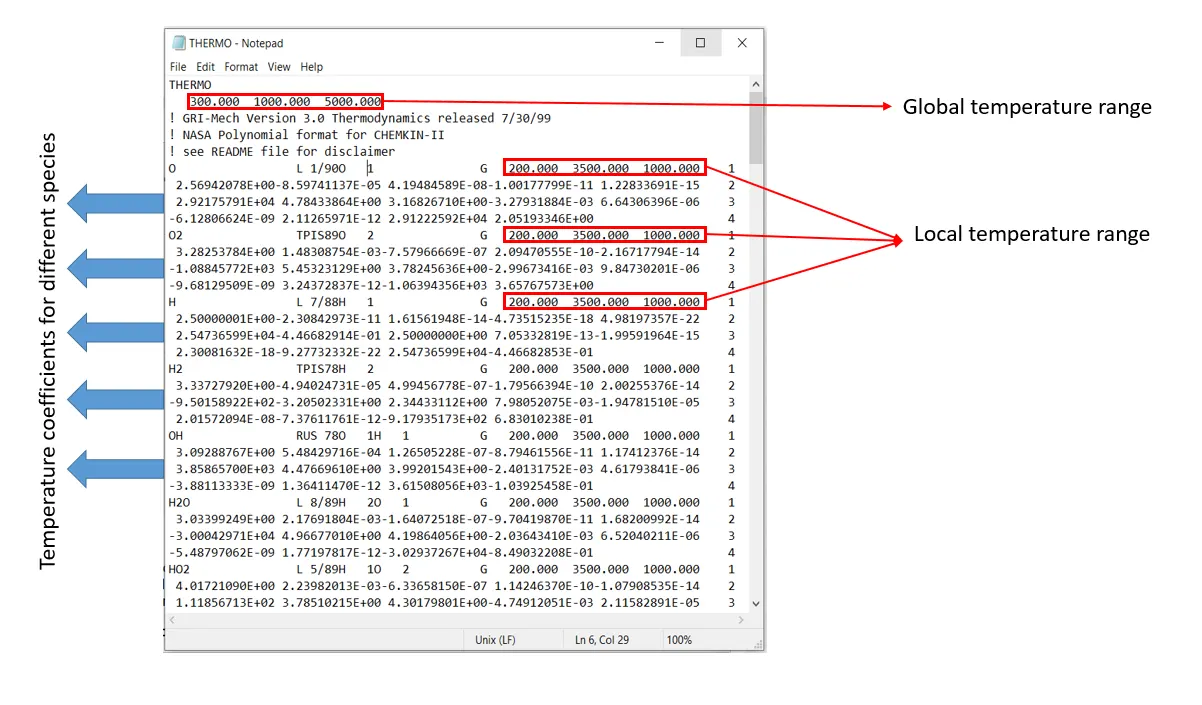 The MATLAB code helps to read the data from the THERMO.dat file which contains temperature ranges, high and low temperature coefficients for different species. These are mentioned in the below figure.
Step-wise approach has been employed to solve this problem. Different steps that are involved in present work are:
- Inputs and outputs in the code:
The only input given in this code is species name. The output that we obtain are plots of thermodynamic properties (specific heat, enthalpy and entropy) across local temperature ranges and molecular weights of different species.
- Extract the high and low temperature coefficients:
As shown in above figure, The NASA thermodynamic dat file contains the temperature coefficients. The first seven temperature coefficients are the high temperature coefficients and remaining are the low temperature coefficients. The high temperature coefficients are considered for solving the thermodynamic equations that have local maximum temperature ranges. Similarly, low temperature coefficients corresponds to local minimum temperature ranges.
To extract this coefficients getl command is used. The co-efficients in that line are spilt and saved in different variables. The coefficients are in form string and to convert them into numerical value str2num command is used.
- Calculation of molecular weights for different species:
Initially the mono atomic weights are given as input such as weights of H, O, C, N, Ar. Using this data the molecules that involves this inputs are made as summation to find the molecular weight of different species.
- Plot and save the graphs in specific species folder:
The thermodynamic properties such as specific heat, enthalpy and entropy across different temperature ranges are plotted using plot command and to these graphs are to be saved in the specific species folder. Let us consider a input species as 'N2'. A folder with species name is created using mkdir command. To save the graphs save as command is used. cd command helps to move this graphs in that particular folder.
- Significance of thermodynamic properties:
These properties helps to find out work expansion or contraction and the type of process i.e.,(reversible or irreversible process). These properties are used to measure the energy of system.
Results:
The following results are obtained from the MATLAB code
- Plots for different species:
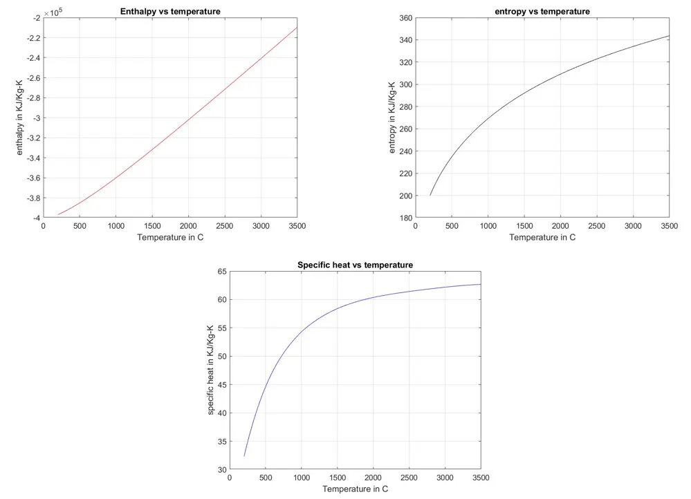
The plots for species CO2, N2 and O2 are presented below. If species input is given as 'CO2'. The plots obtained are:
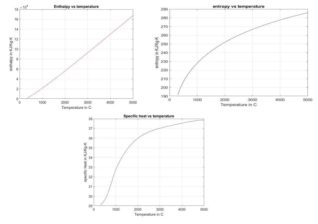
If species input is given as 'N2'. The plots obtained are:
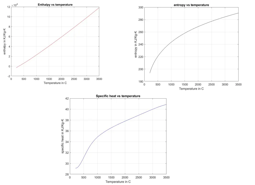
If species input is given as 'O2'. The plots obtained are:
These plots for different species can also be obatined.
- Display of molecular weights in command window:
If the species input is given as O2 then molecular weight (M) is displayed as shown below

If the species input is given as N2 then molecular weight (M) is displayed as shown below

If the species input is given as CO2 then molecular weight (M) is displayed as shown below

- Creating species folder in main folder:
There are different species available in the dat file. The species folders with the element names are created as shown below. In similar way, the other species folders are created. These folders contain the output plots of thermodynamic data.
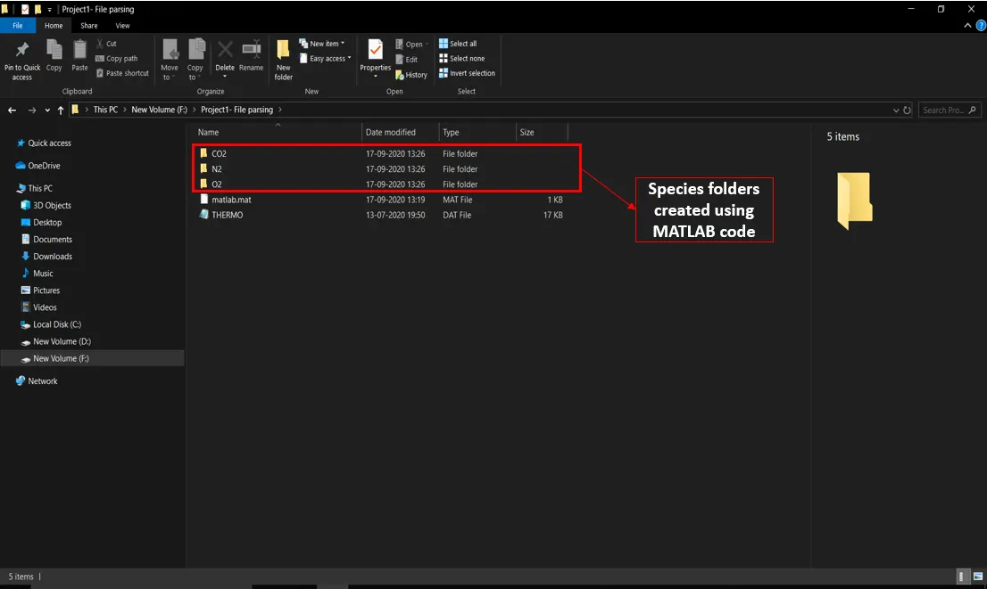
The species folders are saved in the place where the program file is saved.