Project 1 - Parsing NASA thermodynamic data

% parsing NASA thermodynamic data and obtaining results from from it
f = fopen('THERMO.dat', 'r');
fgetl(f); % ignoring the first line as it is just a file name
sl = strtrim(fgetl(f)); % second line
global_temps = strsplit(sl,' ');
global_low_temp = str2double(global_temps{1});
global_mid_temp = str2double(global_temps{2});
global_high_temp = str2double(global_temps{3});

% the next three lines are just comments which can be ignored
for i=1:3
    fgetl(f);
end

l = 1;
% loop for reading all species
while(f>0)
    l = fgetl(f); % this line store the different species each time
    l = strsplit(l,' ');
    if strcmp(l{1},'END')
        break;
    end
    species_name = l{1};
    low_temp = str2double(l{end-3});
    high_temp = str2double(l{end-2});
    mid_temp = str2double(l(end-1));
    temp = [low_temp mid_temp high_temp];
    temp_range = linspace(low_temp, high_temp, 1000);
    temp_coeff = zeros(1,14);
    c=1;
    % loop for reading each coefficients line of the specific species
    for j=1:3
        m = fgetl(f);
        e = strfind(m, 'E');
        temp_coeff(c) = str2double(m(1:e(1)+3));
        c = c+1;
        %
        for n=1:length(e)-1
            temp_coeff(c) = str2double(m(e(n)+4:e(n+1)+3));
            c = c+1;
        end
    end
    %     low_temp_coeff = temp_coeff(8:14); 
    %     % the first 7 values of the temp_coeff are high temp coeff
    %     high_temp_coeff = temp_coeff(1:7);
    %     % the last 7coeff are low temp coeff
    for i=1:length(temp_range)
        [cp, h, s] = thermo_prop(temp_coeff, mid_temp, temp_range);
    end
    
    %changing directory to save plots
    cd('D:matlab filesNASAoutput')
    mkdir(species_name);
    cd(species_name)
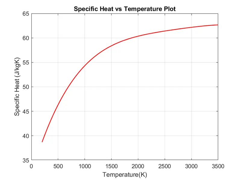
    figure(1)
    plot(temp_range,cp,'linewidth',1.25,'color','r')
    xlabel('Temperature(K)');
    ylabel('Specific Heat (J/kgK)');
    title('Specific Heat vs Temperature Plot')
    grid on
    saveas(figure(1),sprintf('%s.png',sprintf('Specific Heat of %s',species_name)));
    figure(2)
    plot(temp_range,h,'linewidth',1.25,'color','g')
    xlabel('Temperature(K)');
    ylabel('Enthalpy (J/mol)');
    title('Enthalpy vs Temperature Plot')
    grid on
    saveas(figure(2),sprintf('%s.png',sprintf('Enthalpy(H) of %s',species_name)));
    figure(3)
    plot(temp_range,s,'linewidth',1.25,'color','b')
    xlabel('Temperature(K)');
    ylabel('Entropy(J/K)');
    title('Entropy vs Temperature Plot')
    grid on
    saveas(figure(3),sprintf('%s.png',sprintf('Entropy of %s',species_name)));
   
    
    % species{i} = {species_name, low_temp, mid_temp, high_temp, low_temp_coeff, high_temp_coeff,,high_temp)};
    % species cell store species name, local_low_temp, local_high_temp
    % low temperature coeffs and high temperature coeffs respectively.
end
f.close(f);

% this function takes temp coeff and temperature as arguments and returns the value of thermodynamic properties of like 
% speific heat capacity at constant pressure(cp), enthalpy(h) and entropy(s)
function [cp, h, s] = thermo_prop(a, mt, T)
R = 8.314; % universal gas constant
% a is a 1x7 marix which has 7 coefficients
if T<mt
   cp = R.*(a(7+1)+a(7+2)*T+a(7+3)*T.^2+a(7+4)*T.^3+a(7+5)*T.^4);
   h = R.*T.*(a(7+1)+a(7+2)*(T/2)+a(7+3)*((T.^2)./3)+a(7+4)*((T.^3)./4)+a(7+5)*((T.^4)./5)+a(7+6)./T);
   s = R.*(a(7+1)*log(T)+a(7+2)*T+a(7+3)*((T.^2)./2)+a(7+4)*((T.^3)./3)+a(7+5)*((T.^4)./4)+a(7+7));
else
   cp = R.*(a(1)+a(2)*T+a(3)*T.^2+a(4)*T.^3+a(5)*T.^4);
   h = R.*T.*(a(1)+a(2)*(T/2)+a(3)*((T.^2)./3)+a(4)*((T.^3)./4)+a(5)*((T.^4)./5)+a(6)./T);
   s = R.*(a(1)*log(T)+a(2)*T+a(3)*((T.^2)./2)+a(4)*((T.^3)./3)+a(5)*((T.^4)./4)+a(7));
end
end

For O2

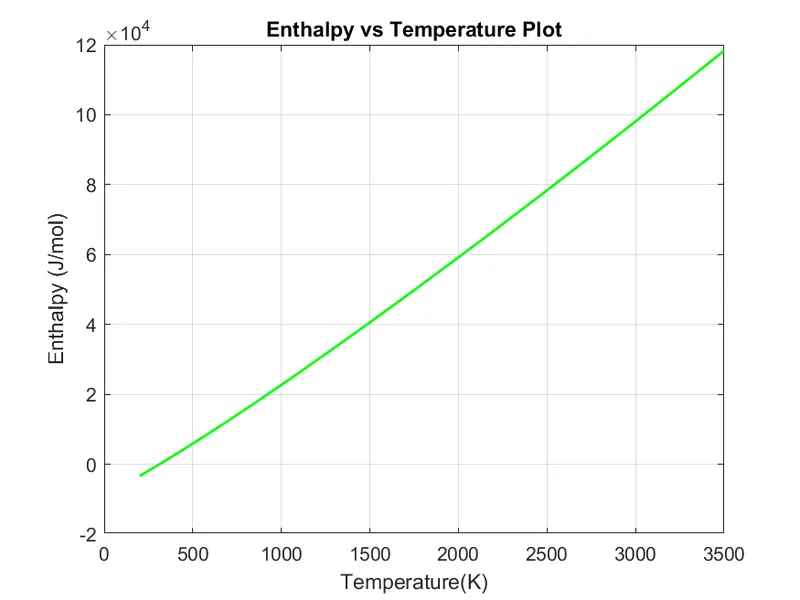
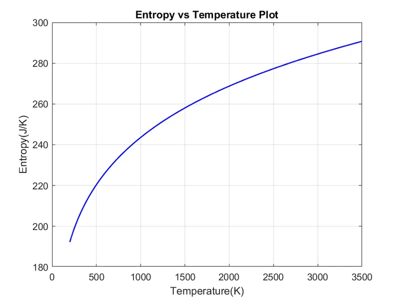
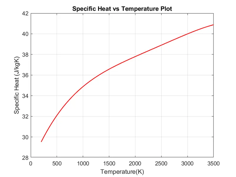
For N2

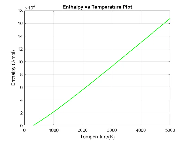
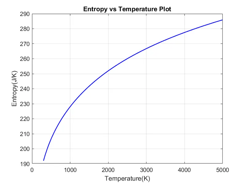
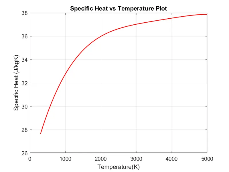
For CO2

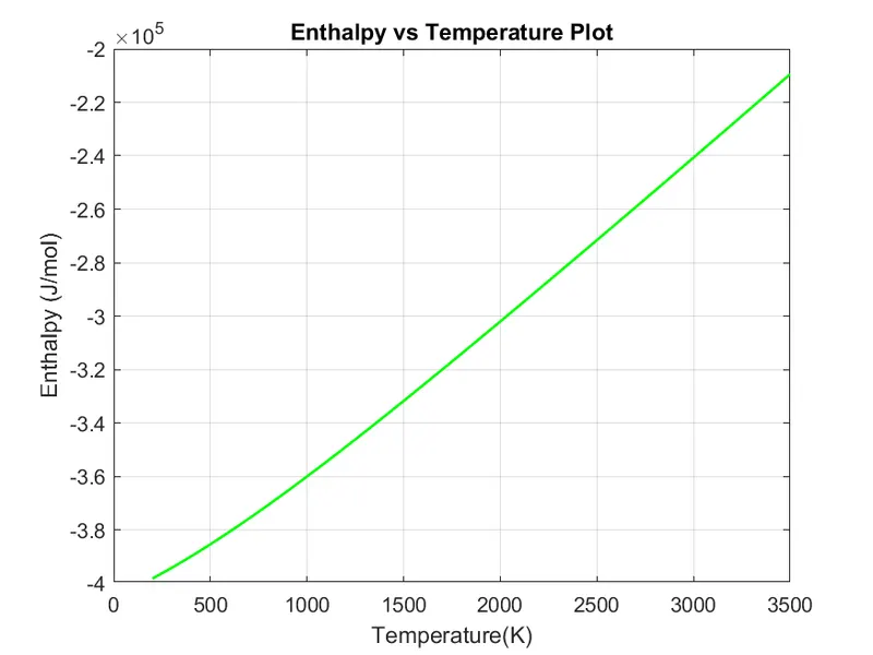
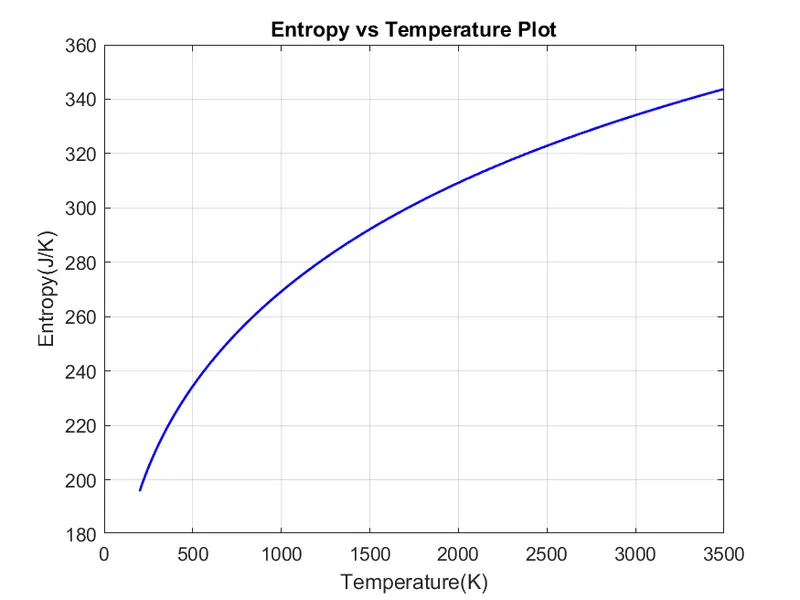
Explanation:

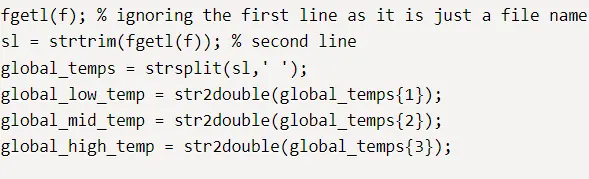
I get the second line of file in sl and store the global temperature values.

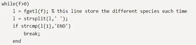
if the species name is 'END' the the loop ends.

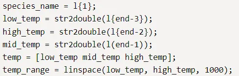
from the first line of species block, species name and local temperatures are stored. A range of temperature values are calculated for plotting the graph from least temperature value to highest temperautre

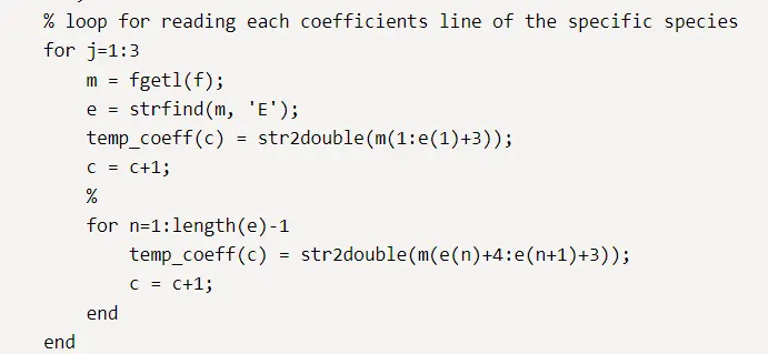
the three lines for temperature coefficients will be calculated. The position of 'E' is utilised to find the values.

thermodynamic properties are calculated for each case of species.

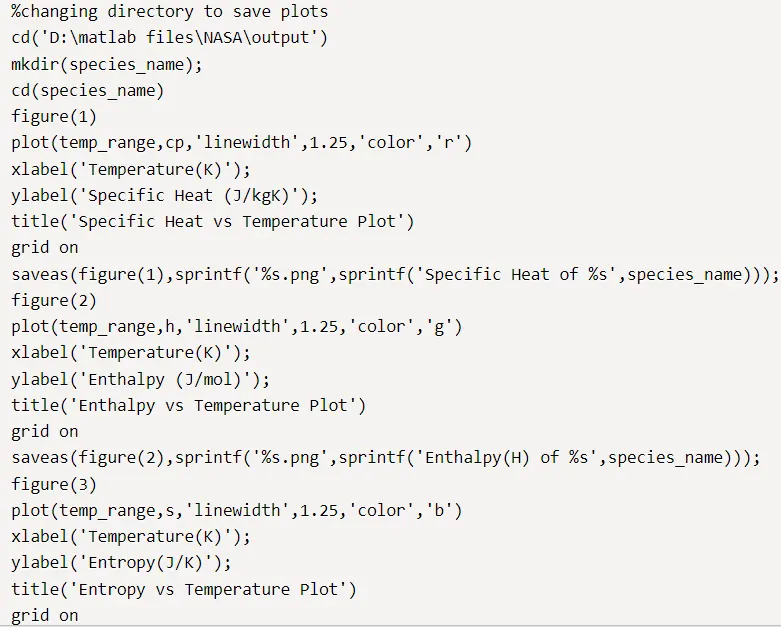
plotting the three graphs for cp, enthalpy and entropy with respect to temperature. The directory is changed each time in the beginning.

the thermo_prop function is used to calculate cp,h,s based on these equations:

here when the temperature is less than mid temperature then the low temperature coefficients are used which are the last seven and the the temperature is higher than mid temperaure then high temperature coefficients are used which are the first seven.