Project 1 - Implement and deploy CNN model in real-time using python on Fashion MNIST dataset

Implement and deploy CNN model in real-time using python on Fashion MNIST dataset

#Importing the libraries

import numpy as np

import pandas as pd

from tensorflow import keras

from tensorflow.keras.utils import to_categorical

from tensorflow.keras.models import Sequential

from tensorflow.keras.layers import Dense,Dropout,Activation,Flatten

from tensorflow.keras.layers import Conv2D,MaxPooling2D,BatchNormalization

from tensorflow.keras.losses import categorical_crossentropy

from sklearn.model_selection import train_test_split

from tensorflow.keras.regularizers import l2

from tensorflow.keras.preprocessing.image import ImageDataGenerator

from sklearn.metrics import accuracy_score,classification_report,confusion_matrix

import matplotlib.pyplot as plt

import seaborn as sns

import warnings

warnings.filterwarnings('ignore')

#Importing the dataset

train_data = pd.read_csv('fashion-mnist_train.csv')

print(train_data.shape)

test_data = pd.read_csv('fashion-mnist_test.csv')

print(test_data.shape)

train_data.head()

train_data.info()

#Unique values in label column of training dataset

train_data['label'].unique()

#Counting number of images for each label class

train_data['label'].value_counts()

#Separating independent and dependent variables for train and test data

train_x = train_data.drop(columns=['label'])

y_train = train_data['label']

test_x = test_data.drop(columns=['label'])

y_test = test_data['label']

train_x.shape, y_train.shape ,test_x.shape,y_test.shape

#Reshaping the data

x_train = train_x.values.reshape(train_x.shape[0],28,28,1)

x_test = test_x.values.reshape(test_x.shape[0],28,28,1)

print('x_train shape',x_train.shape)

print('x_test shape',x_test.shape)

print('y_train shape',y_train.shape)

feature scaling

• Each image is 28 pixels in height and 28 pixels in width, for a total of 784 pixels in total.
• The 784 pixels columns values in each row contain brightness information for each pixel in the 28x28 grayscale image.
• Each pixel has a single pixel value associated with it, indicating the lightness or darkness of that pixel, with higher numbers meaning darker.
• This pixel value is an integer between 0(black) and 255(white). Values in between represent different shades of gray.
• To normalize the values, we therefore need to divide each pixel cell by 255

#Normalizing train & test data between 0 to 1

x_train = x_train/255

x_test = x_test/255

#Visualizing the images

y_train.unique()

#Numeric labels are not that meaningful in a visualization, we'll map them to a textual representation

#0 => T-shirt/top,1 => Trouser,2 => Pullover,3 => Dress,4 => Coat,5 => Sandal,6 => Shirt,7 => Sneaker,8 => Bag,9 => Ankle boot

class_labels = ['T shirt/top','Trouser','Pullover','Dress','Coat','Sandal','Shirt','Sneaker','Bag','Ankle boot']

#Set figure size

plt.figure(figsize = (10,10))

#Showing randomly 20 images from training dsataset

j=1

for i in np.random.randint(0,6000,20):

plt.subplot(6,5,j)

j+=1

plt.xticks([])

plt.yticks([])

plt.imshow(x_train[i],cmap = plt.cm.binary)

plt.title('{}/{}'.format(class_labels[y_train[i]],y_train[i]))

#Train-test split dataset

x_train,x_val,y_train,y_val = train_test_split(x_train,y_train,test_size = 0.2,random_state=42)

x_train.shape , y_train.shape

x_val.shape , y_val.shape

#Convolutional Neural Network - Model Building

model = keras.models.Sequential([

keras.layers.Conv2D(filters = 32,kernel_size = 3,padding = 'valid',activation = 'relu',input_shape = [28,28,1]),

keras.layers.MaxPooling2D(pool_size = (2,2)),

keras.layers.Conv2D(filters = 64,kernel_size = 3,padding = 'same',activation = 'relu'),

keras.layers.MaxPooling2D(pool_size = (2,2)),

keras.layers.Flatten(),

keras.layers.Dense(units=256, activation='relu'),

keras.layers.Dropout(0.5),

keras.layers.Dense(units = 128,activation = 'relu'),

keras.layers.Dropout(0.10),

keras.layers.Dense(units = 10,activation = 'softmax')])

#Model summary

model.summary()

#Model compile

model.compile(optimizer = 'adam',loss = 'sparse_categorical_crossentropy',metrics = ['accuracy'])

#Train

history = model.fit(x_train,y_train,epochs = 15 ,batch_size = 512,verbose = 1 , validation_data = (x_val,y_val))

#List of all the data in history

print(history.history.keys())

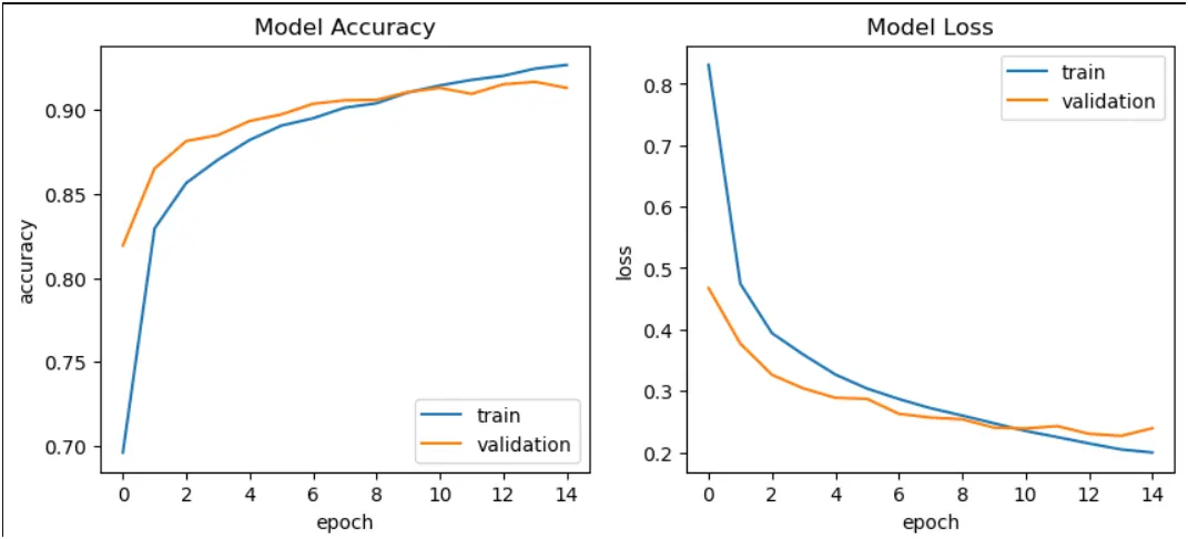
#Plotting accuracy and loss of the model

def plot_training_hist(history):

'''Function to plot history for accuracy and loss'''

fig, ax = plt.subplots(1, 2, figsize=(10,4))

# first plot

ax[0].plot(history.history['accuracy'])

ax[0].plot(history.history['val_accuracy'])

ax[0].set_title('Model Accuracy')

ax[0].set_xlabel('epoch')

ax[0].set_ylabel('accuracy')

ax[0].legend(['train', 'validation'], loc='best')

# second plot

ax[1].plot(history.history['loss'])

ax[1].plot(history.history['val_loss'])

ax[1].set_title('Model Loss')

ax[1].set_xlabel('epoch')

ax[1].set_ylabel('loss')

ax[1].legend(['train', 'validation'], loc='best')

plot_training_hist(history)

#Test Model

np.argmax(model.predict(np.expand_dims(x_test[0],axis = 0)).round(2)) #test on single test image(predicted label)

y_test[0] #actual label of above image

#Testing on all test images

y_pred = model.predict(x_test).round(2)

y_pred

#Model evaluation

model.evaluate(x_test,y_test)

#Visualize output

plt.figure(figsize = (25,30))

#Comparing randomly actual and predicted labels from test data

j=1

for i in np.random.randint(0,1000,20):

plt.subplot(10,5,j);j+=1

plt.xticks([])

plt.yticks([])

plt.imshow(x_test[i].reshape(28,28),cmap = 'Greys')

plt.title('Actual = {} / {} predicted = {} / {}'.format(class_labels[y_test[i]],y_test[i],class_labels[np.argmax(y_pred[i])],np.argmax(y_pred[i])))

#Confusion Matrix

y_predicted_labels = [np.argmax(label) for label in y_pred]

cm = confusion_matrix(y_test,y_predicted_labels)

print('confusion_matrix:n',cm)

#Plotting the confusion matrix

plt.figure(figsize=(7,5))

sns.heatmap(cm,annot = True,fmt = 'd',xticklabels=class_labels, yticklabels=class_labels)

#Classification report

cl_report = classification_report(y_test,y_predicted_labels , target_names = class_labels)

print(cl_report)

We can say from above report:

• Trouser, Sandal, Bag, Ankle boot model performance is very good.
• Shirt model performance is not very good comparatively.