Project 1 - Data Handling and Interpolation
Project :
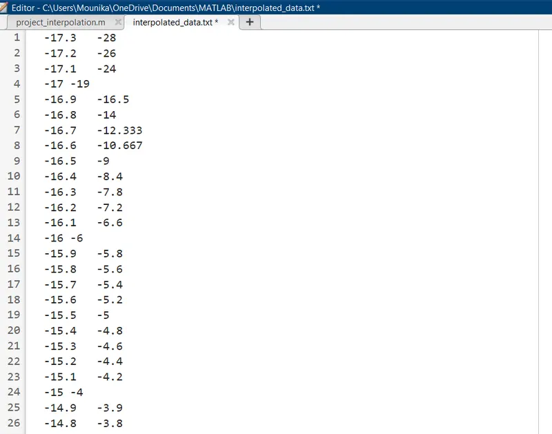
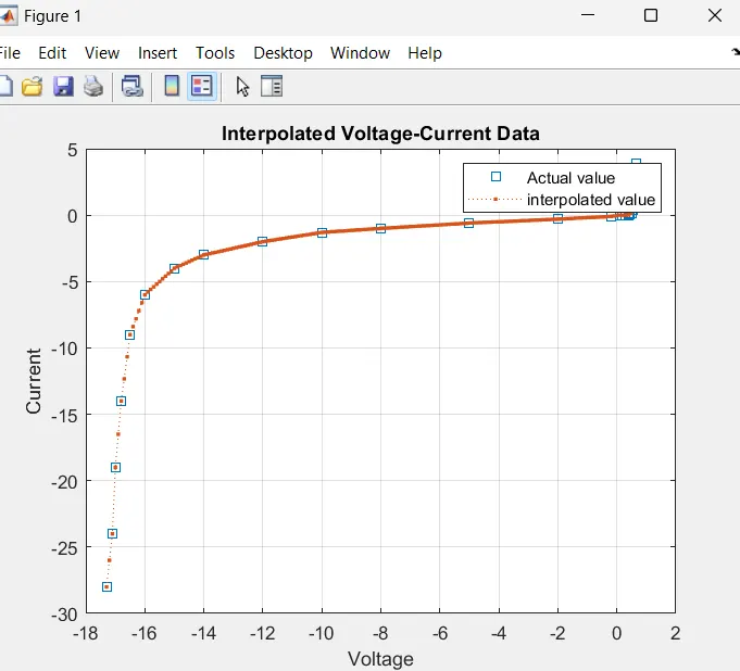
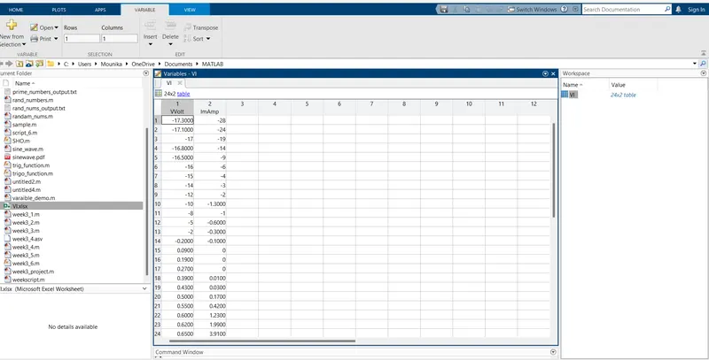
In a laboratory experiment, data of voltage and current has been recorded and the same is attached in an excel file ( Click on this link VI.xlsx ). Read the excel file in the Matlab program and perform the interpolation in the range of -17.3:0.1:0.9. Generate the interactive plot for the interpolated data and store them in a text file.
Key Highlights:
- Graphical solutions are more visual and appealing
- Interpolation of data
- Read excel file
- Write to text file
Deliverables:
- Find missing data and save it in text
- Interpolate the data set
- Save your program and attach the same.
- Save txt file and upload in attachment
AIM:
- To read the excel file in the matlab and performing the interpolation with the given range.
- To generate the interactive plot for the interpolated data and to store them in to a text file.
Answer:-
Defination of interpolation:
Interpolation is the process of estimating the values of a function between known data points. It involves constructing a new function that passes through the given data points and can be used to estimate the value of the function at any point within the interval spanned by the data points.
Methods of interpolation:
There are many interpolation methods but some of the most commonly used methods are given below:
1. Linear Interpolation
2. Nearest Neighbor Interpolation
3. Cubic Interpolation
4. Piecewise Polynomial Interpolation
5. Grid Data Interpolation
6. Custom Interpolation
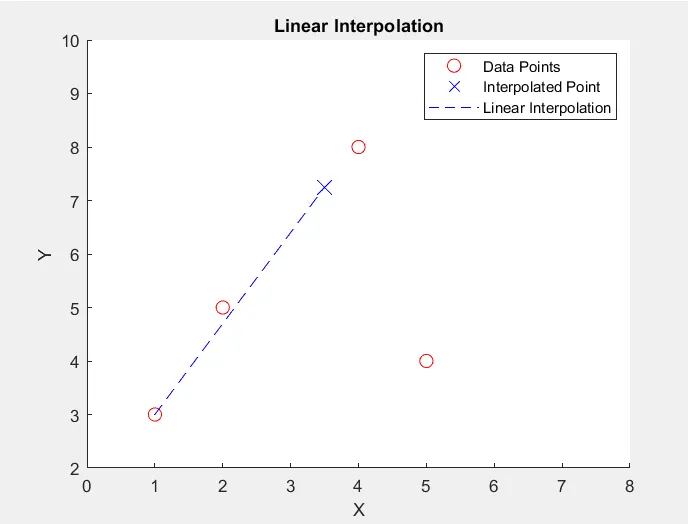
1. Linear Interpolation: Linear interpolation is the simplest form of interpolation. It estimates values between two adjacent data points by assuming a straight line between them. In Matlab, linear interpolation can be performed using the "interp1" function with the interpolation method set to "linear".
example:
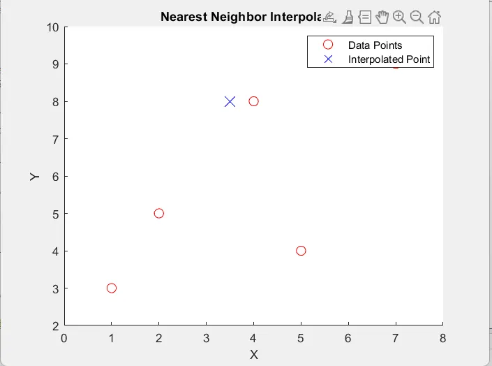
2. Nearest Neighbor Interpolation: Nearest neighbor interpolation assigns the value of the nearest data point to the desired point. In Matlab, nearest neighbor interpolation can be performed using the "interp1" function with the interpolation method set to "nearest".
example:
3. Cubic Interpolation: Cubic interpolation estimates values between data points using cubic polynomials. It provides smoother and more accurate results compared to linear interpolation. In Matlab, cubic interpolation can be performed using the "interp1" function with the interpolation method set to "cubic" or "spline".
example:
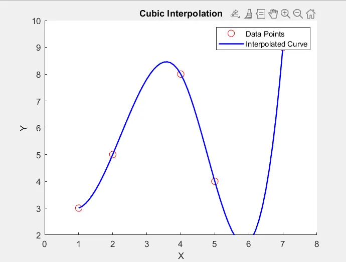
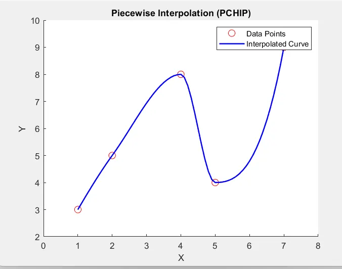
4. Piecewise Polynomial Interpolation: Piecewise polynomial interpolation uses different polynomial functions for different segments of the data. The polynomials are typically higher order (e.g., quadratic or cubic). Matlab provides the "interp1" function with the interpolation method set to "pchip" for piecewise cubic Hermite interpolation or "spline" for piecewise cubic spline interpolation.
example:
5. Grid Data Interpolation: If the data is given on a grid, Matlab provides functions like "interp2" and "interp3" for two-dimensional and three-dimensional interpolation, respectively. These functions use methods such as linear, nearest neighbor, or cubic interpolation to estimate values at points within the grid.
example:
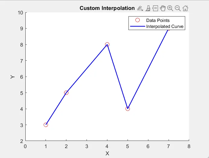
6. Custom Interpolation: Matlab also allows you to define your own custom interpolation methods using the "griddedInterpolant" function. This function lets you specify the interpolation method (e.g., linear, cubic) and other properties to create an interpolant object that can be used for interpolation.
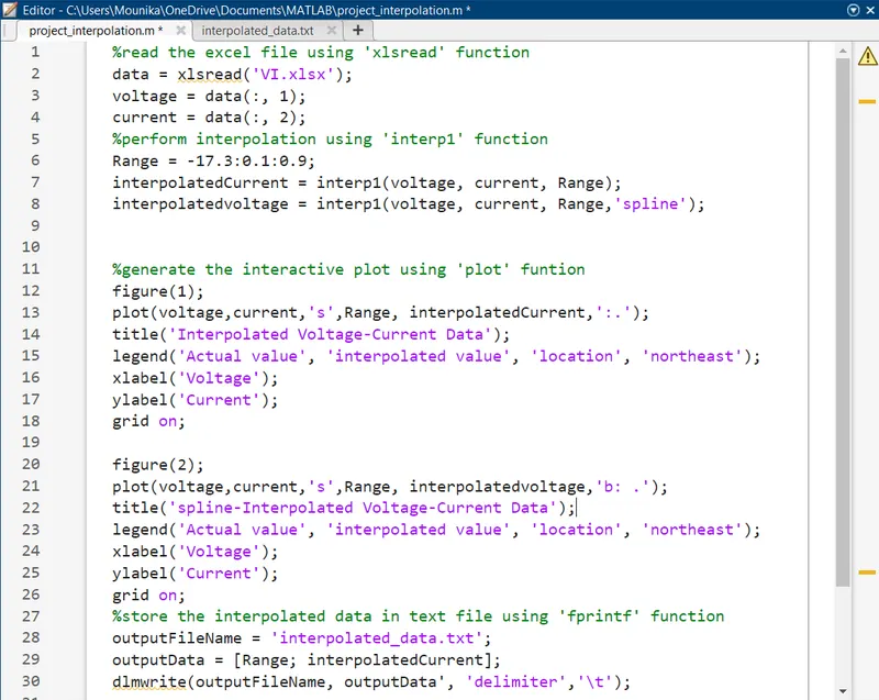
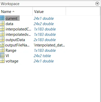
First the data should be recorded from the given excel file,
scriptfile:
%read the excel file using 'xlsread' function
data = xlsread('VI.xlsx');
voltage = data(:, 1);
current = data(:, 2);
%perform interpolation using 'interp1' function
Range = -17.3:0.1:0.9;
interpolatedCurrent = interp1(voltage, current, Range);
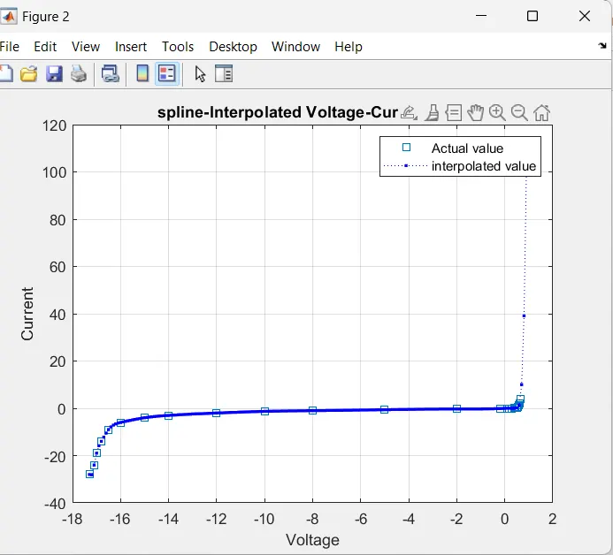
interpolatedvoltage = interp1(voltage, current, Range,'spline');
%generate the interactive plot using 'plot' funtion
figure(1);
plot(voltage,current,'s',Range, interpolatedCurrent,':.');
title('Interpolated Voltage-Current Data');
legend('Actual value', 'interpolated value', 'location', 'northeast');
xlabel('Voltage');
ylabel('Current');
grid on;
figure(2);
plot(voltage,current,'s',Range, interpolatedvoltage,'b: .');
title('spline-Interpolated Voltage-Current Data');
legend('Actual value', 'interpolated value', 'location', 'northeast');
xlabel('Voltage');
ylabel('Current');
grid on;
%store the interpolated data in text file using 'fprintf' function
outputFileName = 'interpolated_data.txt';
outputData = [Range; interpolatedCurrent];
dlmwrite(outputFileName, outputData', 'delimiter','\t');