Project 1 - Data Cleaning and Transformation using Pivot table and Charts for the Report on requirement of Team Hiring

a) Proper Formating

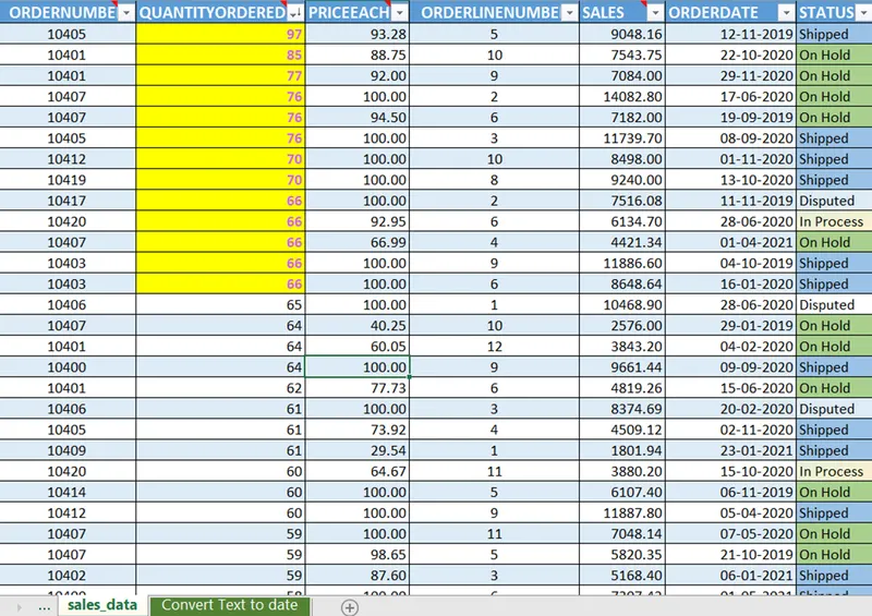
Step1 . Click on a cell with data Insert > Table > confirm default table range is correct ( all data cells are selected) > check My data has headder >OK

Step2. A Default Table design with formatting ( Alternate roww fills) , each column with filters is ready

Step3 . Table Design > Properties > Table Name: > Give a name that suits data or default name is already there.

Step4. Glance your data ( In this case there is Row 2825 that do not carry table data. Delte it.

Step5. Coulmns with only numbers like Ordernumber, Quantity ordered,Orderlinenumber.. are formatted as Numbers with out decimals.

Coulmns with only numbers like Priceeach,Sales,MSRP are formatted as Numbers with two decimals

Coulmns with combinaation of text,numbers and special char like Status, Productline, Customername...are formatted as Strings

Coulmn Orderdate has date and time in different formats. This requires special treatment.

Select all cells in the coulmn (without headding) >Data > Text to Columns >Delimited /Next > TAB and Space checked /Next ( Two coulmns are shown)>Date (DMY) [for first column] >finish -> your Orderdate is now with only date -> Select Full coulmn >Home>Number> Short date.

Ctrl +A Give the disered font /Size.. + First Row > BOLD /size increased by 4 points + All borders.

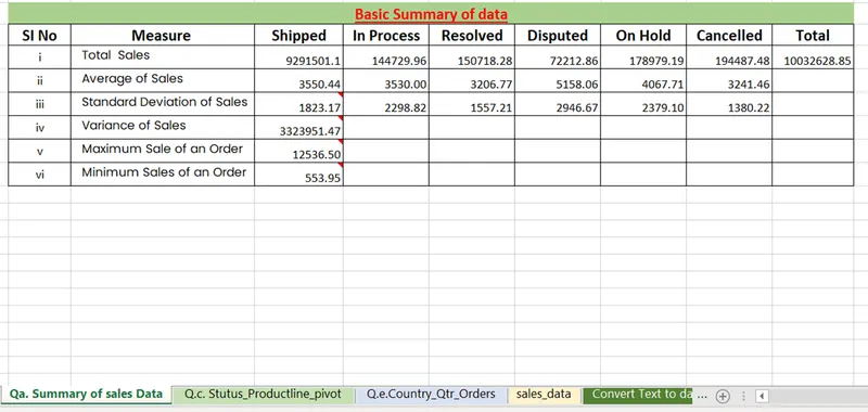
Qb. As Sales depends on Status of the Order ie Shipped, In Process... A table of desired summeries using SUMIF,AVERAGEIF, Array application (CTRL+SHFT+ENT) for STDV.P,VAR.P,MAX and MIN() functions are used and a tabel is creted

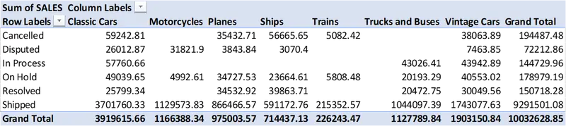
Qc.Using A Pivot table A sheet for comparision of Product Status for different product lines total sales is made

Insert > Pivot Table (While a cell with data is selected) > default [sales_data ]is displayed / check newsheet > OK.

A pivot table in a new work sheet is created with Data fields displayed > Status to Rows > Sales to Valus > Productline to Columns > A beautiful table is created.

PivotTable Analyse > Field Headers (Toggle the icon) >Desired style of Table

Qd.File > OPtions> Customize Ribbons >New Tab > Right click >Rename>ABC[select desired ICon] >New Group (while ABC is Selected)>Choose the shortcuts or add more groups to add all functionality of DATA tab

Qe. Done

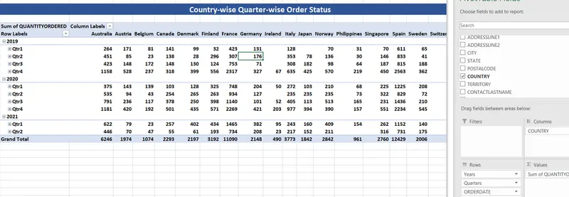
Qf. done. -> Excel Book " proj1_sales_data_answered > Worksheet " sales_data"

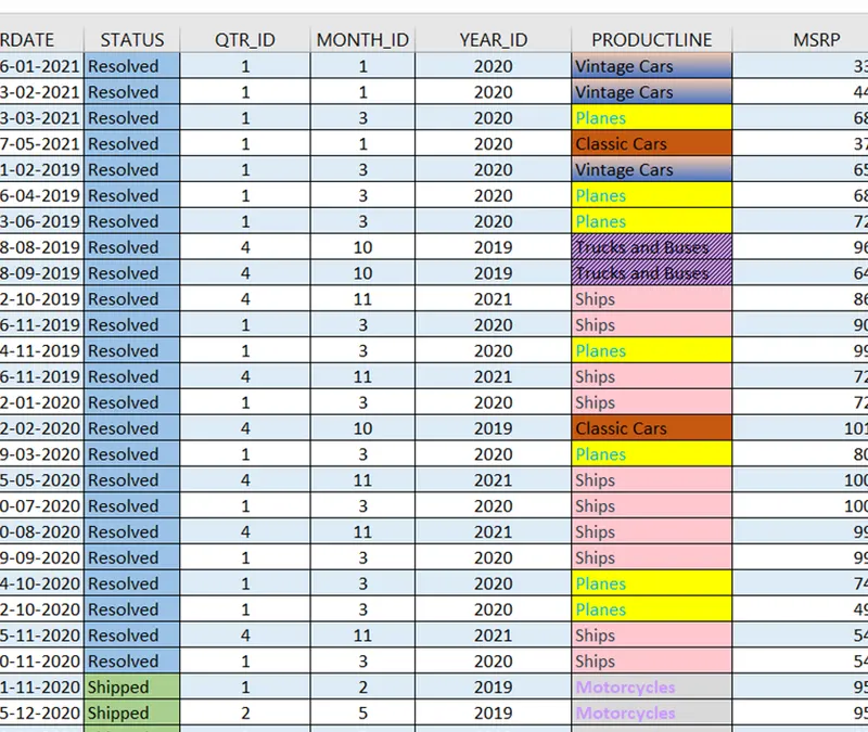
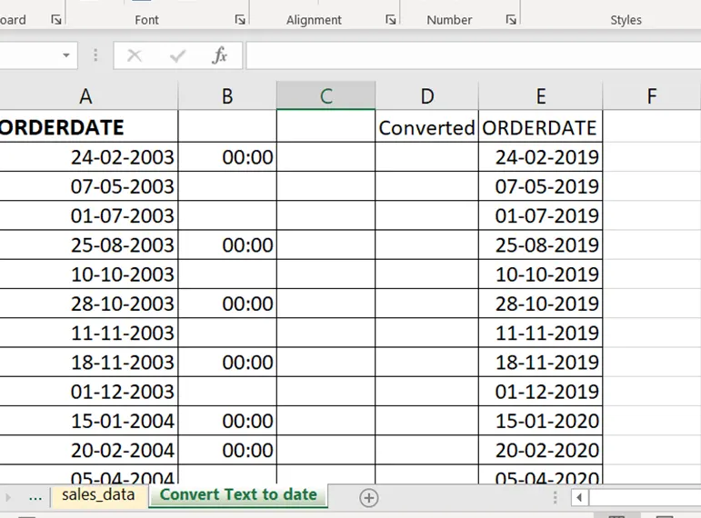
Qg. Data with respect to date is cleaned using date(y,m,d) function and assigned "Short date format" converted with nested if statements to alter year eg 2003 to 2019 -> WorkBook "proj1_sales_data_answered -> sheet "Convert Text to date ".

Qh. Total sales for Orders under differen status are tabulated using SUMIF() function -> WorkBook " proj1_sales_data_answered > Sheet "Qa. Summary of sales Data

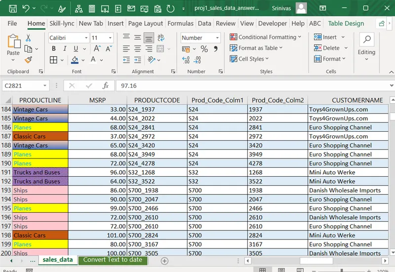
Qi. Insert two columns next to " PRODUCTCODE( we want to split)" Select all cells in the coulmn (without headding) >Data > Text to Columns >Delimited /Next > TAB and Other checked >enter _(Under score) /Next ( Two coulmns are shown)>finish > Select yes for insirting in the sheet -> your Orderdate is now with two new coulmns. Name them as you require, In this case study Prod_Code_Colm1 and Prod_Code_Colm2.

Qj.TOp 10 Orders in the table is Formatted

Select the range to format > Home ribbon > Styles tab > Conditional Formatting >Top > Bottom 10 Rules > Top 10 items > Select the desired formating style >ok