Creating your own openFOAM solver
Objective: -
Create an OpenFOAM solver for scalar transport.
Methodology: -
We will be creating an OpenFOAM solver by customizing an already existing solver called icoFoam. We will be adding additional scalar equations to the solver and validating it with a case pertaining to the same. The post-processing of the simulation will be done through Paraview.
Solver Literature: -
IcoFoam is a solver endemic to OpenFoam which solves the incompressible laminar Navier-Stokes equations using the Pressure Implicit with Settling of Operators (PISO) algorithm. Algorithms like SIMPLE and PISO are used due to the lack of any transport equation for pressure. This project will be an attempt to add scalar transport utility to the current icoFoam solver.
Solver Initialization:
We initialize the solver with four important steps which are adding the scalar transport equations to the core solver code (scalarFoam.C), adding the necessary fields (scalars, vectors, etc ) to the fields directory file (createFields.H), changing the make files and options which contain the instructions for the wmake compilation command and finally running wmake which initializes, compiles and appends the solver to the OpenFoam environment.
scalarFoam.C :
In the source code file, after line 115 where the PISO loop ends, we will be adding our Passive scalar transport equation to the solver to make it our scalarFoam solver. The code is given below:
// Passive Scalar Transport Equation
        fvScalarMatrix sEqn
        (
             fvm::ddt(s)             // Temporal Term
           + fvm::div(phi, s)        // Convection Term
           - fvm::laplacian(su, s)   // Diffusion Term
        );

        sEqn.relax();
        sEqn.solve();
It is important to note that we have to change, add the s to the Eqn objects so that the solver knows we are solving for the scalar s.
createFields.H :
This file acts as the dictionary for our IOobjects which are used in the solver and have to further specify them in the upcoming initial conditioning of the test case.
We are adding the viscosity field for our scalar s which in this case is initialized and declared as su acting as the diffusion coefficient.
dimensionedScalar su
(
    "su",
    dimViscosity,
    transportProperties.lookup("su")
);
In the following code, we are creating our scalar field s which is to be transported, and specifying the arguments that have to be taken for the IOobject and the mesh object.
Info<< "Reading field s \n" << endl;
volScalarField s
(
    IOobject
    (
        "s",
        runTime.timeName(),
        mesh,
        IOobject::MUST_READ,
        IOobject::AUTO_WRITE
    ),
    mesh
);
make/files:
Since we are creating our solver based on the icoFoam solver, we will be making changes to the make files. These files act as the source for compiling our customized solver.
In the files file, we name our solver scalarFoam and specify the solver source code. We further specify the binary location for this solver for the OpenFOAM environment which is in the FOAM_USER_APPBIN. We use this directory for saving customized solvers and testing them.
scalarFoam.C

EXE = $(FOAM_USER_APPBIN)/scalarFoam
make/options:
In the options file, we specify the libraries and the dependencies which are used for our current solver.
EXE_INC = \
    -I$(LIB_SRC)/finiteVolume/lnInclude \
    -I$(LIB_SRC)/meshTools/lnInclude

EXE_LIBS = \
    -lfiniteVolume \
    -lmeshTools
After setting up these files, we finally run the command wmake to compile and initialize our solver.
Test Case:
Since we have successfully compiled our solver, we will be validating it by testing it with a sample case. For this scenario, we will be utilizing the Lid-driven cavity tutorial case which can be found in the tutorials directory of OpenFOAM. We will be naming the solver as scalarCavity. The main purpose of this simulation is to observe the behavior of the scalar s in a domain with a fixed bottom wall and a moving top wall.
Pre-Processing:
We will now be setting up the files which the case takes as input for the simulation. The general system of the input files is organized into three folders namely 0, constant, and system. We will be looking at each file as we chronologically move on.
0/p:
0 contains the initial scalar and vector fields to be taken like pressure, velocity, etc. The following shows the scalar data for the pressure file p.
/*--------------------------------*- C++ -*----------------------------------*\
  =========                 |
  \\      /  F ield         | OpenFOAM: The Open Source CFD Toolbox
   \\    /   O peration     | Website:  https://openfoam.org
    \\  /    A nd           | Version:  8
     \\/     M anipulation  |
\*---------------------------------------------------------------------------*/
FoamFile
{
    version     2.0;
    format      ascii;
    class       volScalarField;
    object      p;
}
// * * * * * * * * * * * * * * * * * * * * * * * * * * * * * * * * * * * * * //

dimensions      [0 2 -2 0 0 0 0];

internalField   uniform 0;

boundaryField
{
    movingWall
    {
        type            zeroGradient;
    }

    fixedWalls
    {
        type            zeroGradient;
    }

    frontAndBack
    {
        type            empty;
    }
}

// ************************************************************************* //
0/s:
The following file shows the data for our scalar s. Since it is dimensionless, we have specified all zero values.
/*--------------------------------*- C++ -*----------------------------------*\
  =========                 |
  \\      /  F ield         | OpenFOAM: The Open Source CFD Toolbox
   \\    /   O peration     | Website:  https://openfoam.org
    \\  /    A nd           | Version:  8
     \\/     M anipulation  |
\*---------------------------------------------------------------------------*/
FoamFile
{
    version     2.0;
    format      ascii;
    class       volVectorField;
    object      s;
}
// * * * * * * * * * * * * * * * * * * * * * * * * * * * * * * * * * * * * * //

dimensions      [0 0 0 0 0 0 0];

internalField   uniform (0 0 0);

boundaryField
{
    movingWall
    {
        type            zeroGradient;
    }

    fixedWalls
    {
        type            zeroGradient;
    };
    }

    frontAndBack
    {
        type            empty;
    }
}

// ************************************************************************* //
0/U:
The following file shows the vector data for the velocity U.
/*--------------------------------*- C++ -*----------------------------------*\
  =========                 |
  \\      /  F ield         | OpenFOAM: The Open Source CFD Toolbox
   \\    /   O peration     | Website:  https://openfoam.org
    \\  /    A nd           | Version:  8
     \\/     M anipulation  |
\*---------------------------------------------------------------------------*/
FoamFile
{
    version     2.0;
    format      ascii;
    class       volVectorField;
    object      U;
}
// * * * * * * * * * * * * * * * * * * * * * * * * * * * * * * * * * * * * * //

dimensions      [0 1 -1 0 0 0 0];

internalField   uniform (0 0 0);

boundaryField
{
    movingWall
    {
        type            fixedValue;
        value           uniform (1 0 0);
    }

    fixedWalls
    {
        type            noSlip;
    }

    frontAndBack
    {
        type            empty;
    }
}

// ************************************************************************* //
constant/transportProperties:
The constant directory consists of the dictionary transportProperties which acts as a library of models for viscosity. In our case, we have the Newtonian model dimensionedScalar `nu`(nu) with a value of 0.01 and our custom dimensionedScalar su with the value 0.001.
/*--------------------------------*- C++ -*----------------------------------*\
  =========                 |
  \\      /  F ield         | OpenFOAM: The Open Source CFD Toolbox
   \\    /   O peration     | Website:  https://openfoam.org
    \\  /    A nd           | Version:  8
     \\/     M anipulation  |
\*---------------------------------------------------------------------------*/
FoamFile
{
    version     2.0;
    format      ascii;
    class       dictionary;
    location    "constant";
    object      transportProperties;
}
// * * * * * * * * * * * * * * * * * * * * * * * * * * * * * * * * * * * * * //

nu              [0 2 -1 0 0 0 0] 0.01;
su              [0 2 -1 0 0 0 0] 0.0001;


// ************************************************************************* //
system/blockMeshDict:
In OpenFOAM, the mesh is generated from the data specified in the blockMeshDict file. In our case, we are specifying 60 cells in both x and y directions.
/*--------------------------------*- C++ -*----------------------------------*\
  =========                 |
  \\      /  F ield         | OpenFOAM: The Open Source CFD Toolbox
   \\    /   O peration     | Website:  https://openfoam.org
    \\  /    A nd           | Version:  8
     \\/     M anipulation  |
\*---------------------------------------------------------------------------*/
FoamFile
{
    version     2.0;
    format      ascii;
    class       dictionary;
    object      blockMeshDict;
}
// * * * * * * * * * * * * * * * * * * * * * * * * * * * * * * * * * * * * * //

convertToMeters 0.1;

vertices
(
    (0 0 0)
    (1 0 0)
    (1 1 0)
    (0 1 0)
    (0 0 0.1)
    (1 0 0.1)
    (1 1 0.1)
    (0 1 0.1)
);

blocks
(
    hex (0 1 2 3 4 5 6 7) (60 60 1) simpleGrading (1 1 1)
);

edges
(
);

boundary
(
    movingWall
    {
        type wall;
        faces
        (
            (3 7 6 2)
        );
    }
    fixedWalls
    {
        type wall;
        faces
        (
            (0 4 7 3)
            (2 6 5 1)
            (1 5 4 0)
        );
    }
    frontAndBack
    {
        type empty;
        faces
        (
            (0 3 2 1)
            (4 5 6 7)
        );
    }
);

mergePatchPairs
(
);

// ************************************************************************* //
system/controlDict:
The controlDict dictionary acts as the Input/Output database for our simulation in the terms of time which is an inextricable part. This dictionary sets the simulation start and end time, the number of time steps, and the intervals at which data has to be saved which will be post-processed for visualization. In our case, we have taken an end time of 2 seconds with time steps of 1e-4 and writeInterval of 20. It is also important to specify our solver (scalarFoam) in the application.
/*--------------------------------*- C++ -*----------------------------------*\
  =========                 |
  \\      /  F ield         | OpenFOAM: The Open Source CFD Toolbox
   \\    /   O peration     | Website:  https://openfoam.org
    \\  /    A nd           | Version:  8
     \\/     M anipulation  |
\*---------------------------------------------------------------------------*/
FoamFile
{
    version     2.0;
    format      ascii;
    class       dictionary;
    location    "system";
    object      controlDict;
}
// * * * * * * * * * * * * * * * * * * * * * * * * * * * * * * * * * * * * * //

application     scalarFoam;

startFrom       startTime;

startTime       0;

stopAt          endTime;

endTime         2;

deltaT          1e-4;

writeControl    timeStep;

writeInterval   20;

purgeWrite      0;

writeFormat     ascii;

writePrecision  6;

writeCompression off;

timeFormat      general;

timePrecision   6;

runTimeModifiable true;


// ************************************************************************* //
system/fvSchemes:
The fvSchemes dictionary sets the numerical schemes for terms that are calculated in the simulation. So we specify the numerical schemes for the additional terms which we have added for our scalar transport equation. We are using Gauss Upwind for the divergence term (fvm::div(phi, s)) and Gauss Linear Corrected for the Laplacian term (fvm::laplacian(su, s)).
/*--------------------------------*- C++ -*----------------------------------*\
  =========                 |
  \\      /  F ield         | OpenFOAM: The Open Source CFD Toolbox
   \\    /   O peration     | Website:  https://openfoam.org
    \\  /    A nd           | Version:  8
     \\/     M anipulation  |
\*---------------------------------------------------------------------------*/
FoamFile
{
    version     2.0;
    format      ascii;
    class       dictionary;
    location    "system";
    object      fvSchemes;
}
// * * * * * * * * * * * * * * * * * * * * * * * * * * * * * * * * * * * * * //

ddtSchemes
{
    default         Euler;
}

gradSchemes
{
    default         Gauss linear;
    grad(p)         Gauss linear;
}

divSchemes
{
    default         none;
    div(phi,U)      Gauss linear;
    div(phi,s)      Gauss upwind;
}

laplacianSchemes
{
    default         Gauss linear corrected;
}

interpolationSchemes
{
    default         linear;
}

snGradSchemes
{
    default         orthogonal;
}


// ************************************************************************* //
system/fvSolutions:
The fvSolutions dictionary acts as the solution and algorithm control. It specifies the linear solver (referring to a method to solve matrix equations) that is used for each discretized equation. It also provides the tolerances for each said solver. For our scalar s, we have provided the solver smoothsolver which uses a smoother and tolerance of 1e-5.
/*--------------------------------*- C++ -*----------------------------------*\
  =========                 |
  \\      /  F ield         | OpenFOAM: The Open Source CFD Toolbox
   \\    /   O peration     | Website:  https://openfoam.org
    \\  /    A nd           | Version:  8
     \\/     M anipulation  |
\*---------------------------------------------------------------------------*/
FoamFile
{
    version     2.0;
    format      ascii;
    class       dictionary;
    location    "system";
    object      fvSolution;
}
// * * * * * * * * * * * * * * * * * * * * * * * * * * * * * * * * * * * * * //

solvers
{
    p
    {
        solver          PCG;
        preconditioner  DIC;
        tolerance       1e-06;
        relTol          0.05;
    }

    s
    {
        solver          smoothSolver;
        smoother        symGaussSeidel;
        tolerance       1e-05;
        relTol          0;
    }

    pFinal
    {
        $p;
        relTol          0;
    }

    U
    {
        solver          smoothSolver;
        smoother        symGaussSeidel;
        tolerance       1e-05;
        relTol          0;
    }
}

PISO
{
    nCorrectors     2;
    nNonOrthogonalCorrectors 0;
    pRefCell        0;
    pRefValue       0;
}


// ************************************************************************* //
system/setFieldsDict:
The utility setFieldsDict is used to set values on a selected set of cells/patch-faces in the domain. In our case, we are creating a sphere in the center of the domain where we will calculate and observe the effect of the scalar s.
/*--------------------------------*- C++ -*----------------------------------*\
  =========                 |
  \\      /  F ield         | OpenFOAM: The Open Source CFD Toolbox
   \\    /   O peration     | Website:  https://openfoam.org
    \\  /    A nd           | Version:  8
     \\/     M anipulation  |
\*---------------------------------------------------------------------------*/
FoamFile
{
    version     2.0;
    format      ascii;
    class       dictionary;
    location    "system";
    object      setFieldsDict;
}
// * * * * * * * * * * * * * * * * * * * * * * * * * * * * * * * * * * * * * //

defaultFieldValues
(
    volScalarFieldValue s 0
);

regions
(
    sphereToCell
    {
        centre (0.05 0.05 0);
        radius 0.03;

        fieldValues
        (
            volScalarFieldValue s 1
        );
    }
);


// ************************************************************************* //
Simulation:
To run the simulation, we follow it in three steps using the following commands:
blockMesh : This command initializes and creates our control volume with the mesh.
setfields : This command initializes the dimension of the field s with the given parameters in the setFieldsDict.
scalarFoam : This command finally runs our solver and finishes the simulation from its inception.
Post-Processing:
Once the simulation has been successfully executed, we use the Paraview platform for visualizing the data. For this, we use the command touch scarcavity.foam which creates an input file for Paraview. We then open Paraview and load the foam file we just created. Let's look at the visualized results which show the changes in the scalar s with the elapsed time.
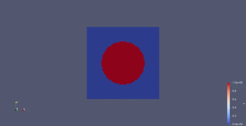
0 seconds
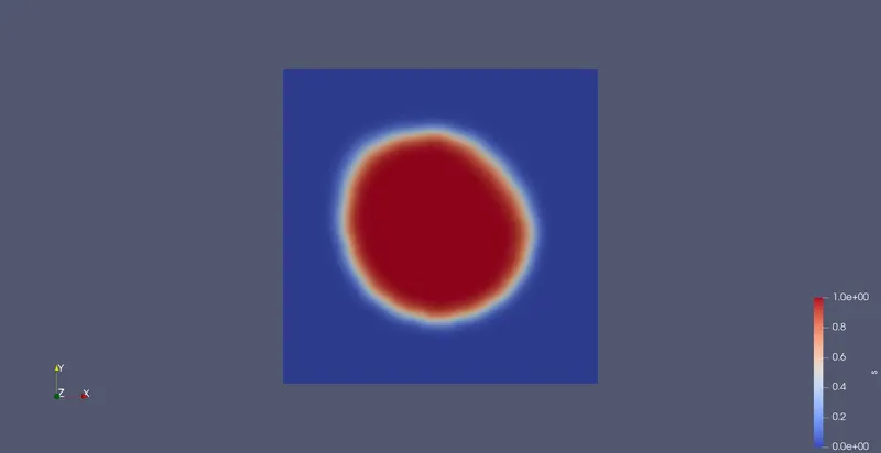
0.02 seconds
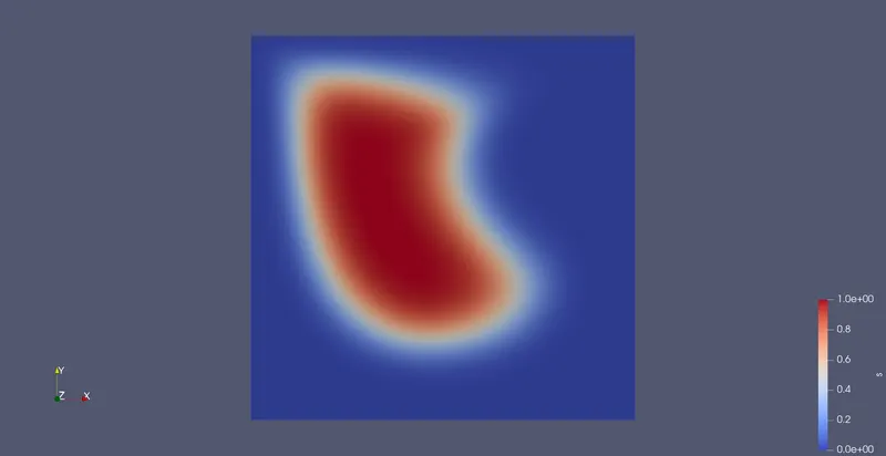
0.1 seconds
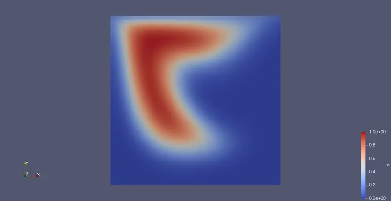
0.2 seconds
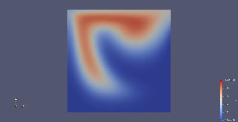
0.3 seconds
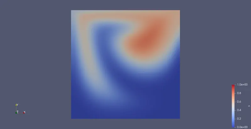
0.4 seconds
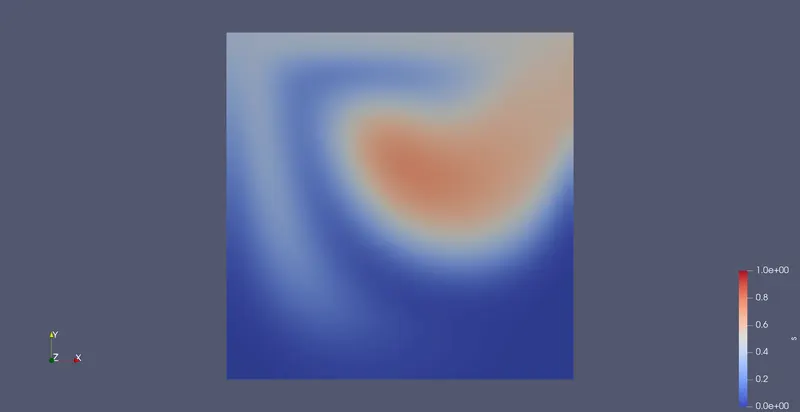
0.5 seconds
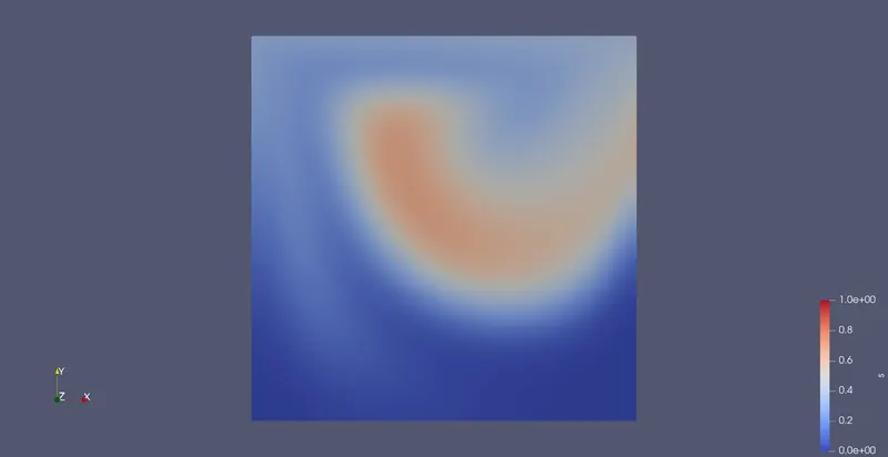
0.6 seconds
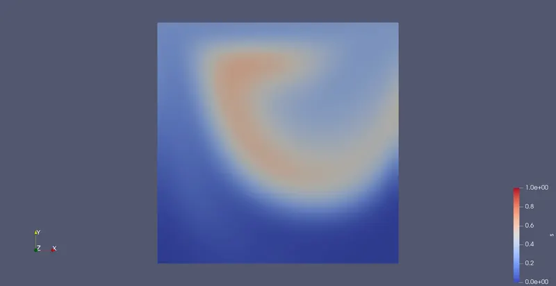
0.7 seconds
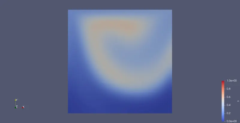
0.8 seconds
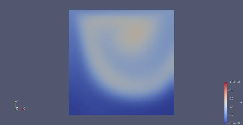
0.9 seconds
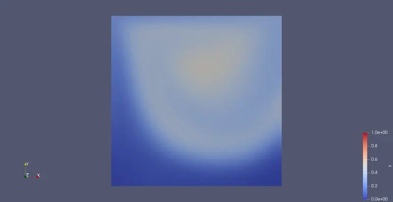
1.0 seconds
Observations and Inference:-
We can see the change in our scalar s with time. Due to the top moving wall, the scalar s is slowly smearing away.
We have seen how to add additional equations (in our case, Passive scalar transport equation) to the existing icoFoam solver and create our own customized solver. And we have validated it with the cavity test case.
This simulation was performed using Ubuntu in Windows Sub System for Linux utility in a Windows 10 system.
References:
https://www.youtube.com/watch?v=L94iYGvZr9Q&list=WL&index=4&ab_channel=8thFloorCFD%40FSB