Project 1- Conjugate Heat Transfer Analysis on a graphics card.

Introduction:

In this project, we will see the conjugate heat transfer analysis of a Graphic Card.Graphic Card is very essential component in different types of computers. Graphic Cards are very efficient for running software and also plays very important role for different kinds of graphics in computers. And for this type of work, it consumes power. And during consumption of power and running for different purposes, it generates heat.This heat generation must be within certain limit for keeping them safe, and for that, always there is a cooling system to maintain its temperature level. Otherwise they may fail. Now, for better product, it is necessary to do an analysis and then based on that report, one can build a graphic card of good quality, which can run so long and keep system running at their optimum condition.

About CHT (Conjugate Heat Transfer) analysis:

Ø Conjugate heat transfer represents combination of heat transfer in both solid and liquids simultaneously. The mode of heat transfer in solids is conduction and in case of liquid it is convection.

Ø Heat transfer in solids is calculated by Fourier’s law, which involves heat transfer only by means of conduction.

Ø For liquids, it is difficult to determine heat transfer because the heat is transported along with the flow of liquid. Sometimes conductive mode of heat transfer dominated the convective heat transfer.

Ø In viscous models, a viscous effect contributes for heat transfer.

Ø In compressible flow, heat generation is fluctuating due to variations in thermal properties of fluid.

About Analysis Model:

Here we have Graphic Card model or model of Unit of GPU on which heat will be applied as a heat generation source, while containing an enclosure around it. Air as a fluid will be passed over it at certain velocity and heat generation through processor and heat dissipation through the fins will be observed. Also we will observe the heat transfer through processor and fins and cooling of unit through the air flow.

Graphic Card Unit:

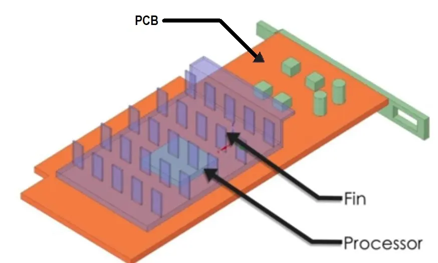
As shown in above image, we have taken a simplified model of graphic card model.In which, main parts are processor, fins and PCB (Printed Circuit Board).There are some other components also fixed on the PCB in this model.

Material Specifications:

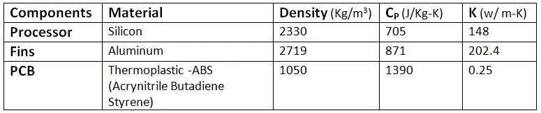
Different materials of components and their properties are given as below:

Fluid Material: Air.

Density = 1.225 (Kg/m³)

C_P =1006.43 (J/Kg-K)

K = 0.0242 (w/ m-K)

Case Approach:

Here we will go through two different cases as Base line Mesh and Refined mesh.

In these cases mainly difference will be regarding the meshing.

Baseline Mesh will be as CASE: M1 and Refined Mesh will be as CASE: M2 created.

Other parameters regarding the simulation will be same for both the cases.

Geometric model with enclosure defined as shown below:

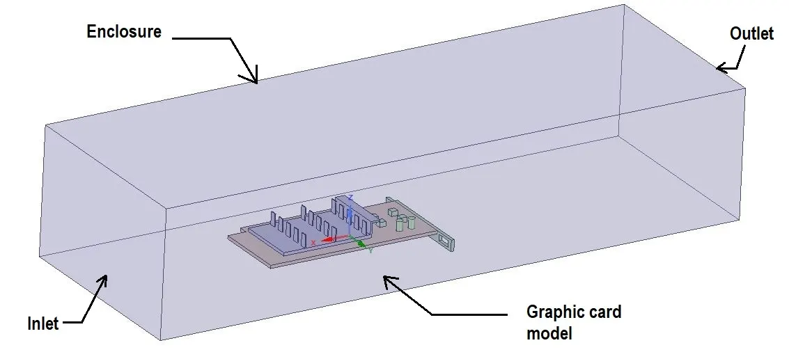
Ø Here in above image we can see the Enclosure and Graphic card model positions.

Ø Inlet and Outlet positions also shown.

Ø Other walls of Enclosure will be taken as symmetric walls.

Meshing Details:

Case	Cell Count	Size	Mesh Refinement
Case : M1	492329	1.6 mm
Case : M2	1205834	8 mm	Body Sizing -Processor: 0.1 mm Body Sizing - Fin : 0.5 mm Body Sizing – PCB : 0.5 mm Inflation: Ø Program Controlled Ø Inflation option: First Layer Thickness Ø First Layer High: 0.1 mm Ø Maximum Layers: 5 Ø Growth Rate: 0.8

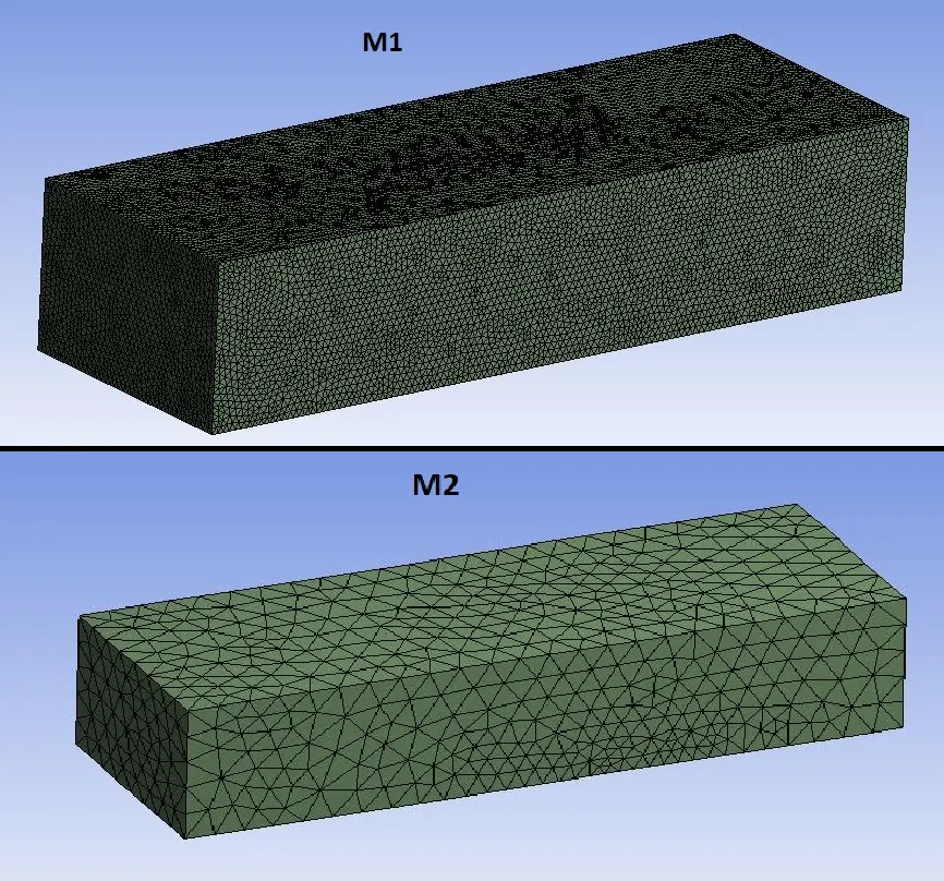
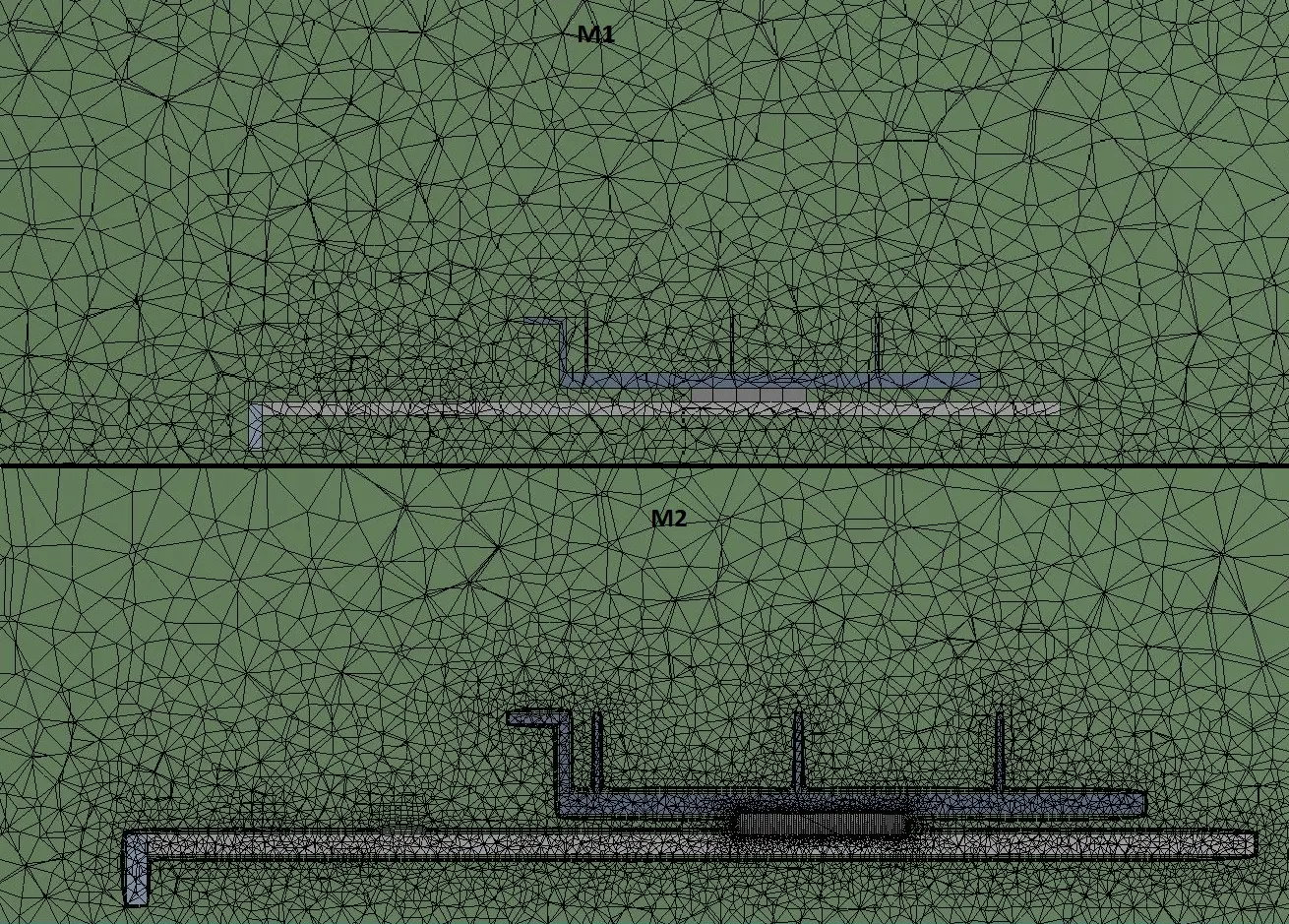
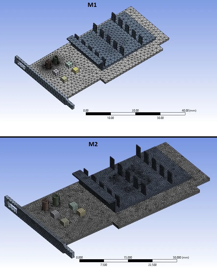
Ø Here In CASE: M1 mesh size is 0.2 mm and in CASE: M2, mesh size is 8 mm.

Where 0.2 mm in CASE: M1 is defined for all components and 8 mm in CASE: M2 is defined for enclosure mesh. It is because of calculation time saving. In CASE: M2 I have refined the mesh for Graphic card components, so the fine mesh for the fluid domain is not needed. So we can create bigger size elements for the fluid domain, because the accuracy is concerned only for the Graphic Card components.

Case Setup Details:

Ø Solver Type : Pressure Based Solver

Ø Energy Equation: On

Ø Viscous Model: K-Epsilon ( Realizable)

Ø Steady State

Boundary Conditions:

Value of Air velocity is based on the Reynolds number.

Up to velocity 7 m/s, the flow ranges from Laminar to transition flow.

From 7.5 m /s, flow becomes Turbulent.

It is Necessary for running the K-Epsilon turbulence model, for solving equation,

that the flow is turbulent.

So, for Reynolds number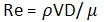

Re = (1.225 * 7.5 * 0.008) / 1.7894 * 10^-5

Re = 4107.522

As we know that after Re = 4000, flow becomes turbulent.

Inlet: Velocity inlet = 7.5 m/s

Outlet: Pressure Outlet = 0 Pa (1 atm)

Temperature for Inlet & Outlet = 293.15 K

Other wall conditions of Enclosure = Symmetric wall

Energy Source: Source term = 156,250,000 w/m³

Ø Here Heat Generation of processor can be standard values referred from the corresponding Graphic card manufacturing companies.

Ø Standard CPU uses between 65 and 85 watts, while quad-core processors range from 95 to 140 watts.

Ø Hard drives may vary greatly according tp age and model; we can get with 10 watts as an estimate, because drives rarely run simultaneously at full load.

So, as per TDP of processor, we can take power consumption or Heat Generation as 10 watts.

Volume V = (8 * 8 * 1) 10^-9 m^3.

So, for the Volumetric Heat Source, Source Term = Heat generated by Processor/ volume

So, Source Term= 10 / 64 * 10^-9

Source Term = 156,250,000 w /m³

---

Procedure:

Ø Import “Graphic Card” file in Ansys SpaceClaim.

Ø After that, on enable the “Share Topology” for all components for conformal Meshing.

Ø Enable the Share Prep for sharing data between Enclosure and Graphic Card components.

Ø Then Create Appropriate Mesh for fluid domain as well as components.

Ø Then run the simulation in the fluent Setup with “Double Precision” and keep parallel processing up to value 4.

Ø Create Material data.

Ø Give boundary conditions to inlet, outlet and walls.

Ø Make sure that all walls and shadows, between all components like processor, fins and PCB are thermally coupled.

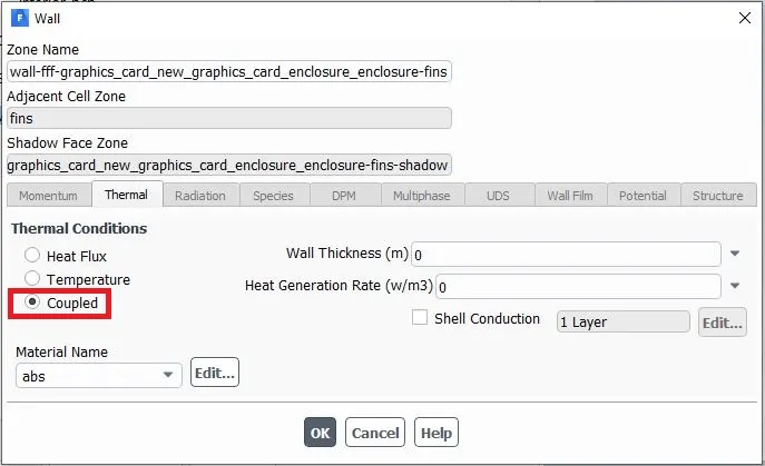
In above image, the condition “Coupled” is marked.

Ø After creating proper reports definitions, initialize with Hybrid Initialization.

Ø Create appropriate Plane for measuring contours.

Ø Create Animations regarding temperature and velocities.

Ø Run the simulations up to convergence.

---

Comparison of Meshing:

Comparison of meshing in both the cases M1 and M2 as given below:

(1)

(2)

(3)

---

Comparison of Results:

Case: M1

Residuals:

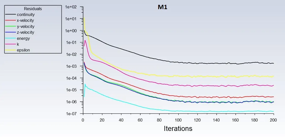
Ø Near about 120 it converges.

Static Temperature:

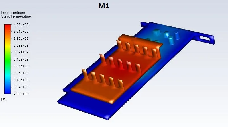
Ø From above plot, 402-293 = 109. So, 273-109=164.

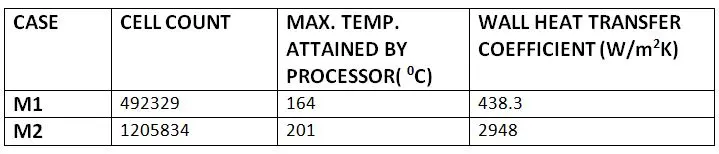
Ø Maximum temperature attained by processor is 164 ⁰C.

Total Temperature:

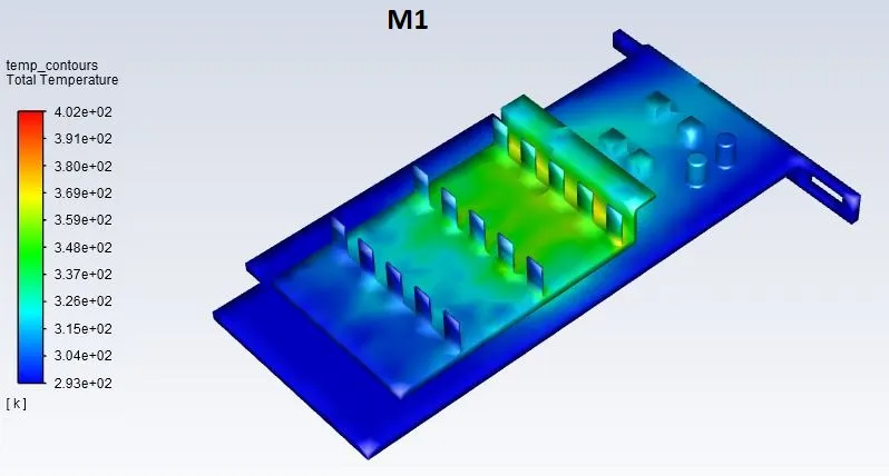
Ø Total temperature includes static temperature and dynamic component related to the kinetic energy of air.

Ø Here we can see the effect of flowing air to the fins.

Ø As shown in above image, as the air passes over the fins, it cools the components.

Ø We can observe that in the starting portion of fins are cooled by air and as it passes, the temperature is high at the rear portion of the fins.

Ø It looks natural that front portion of fins is more cooled then rear portion.

Ø We can clearly see the stagnation of air at the rear portion of fins, and so the temperature is high in that area.

Average Temperature:

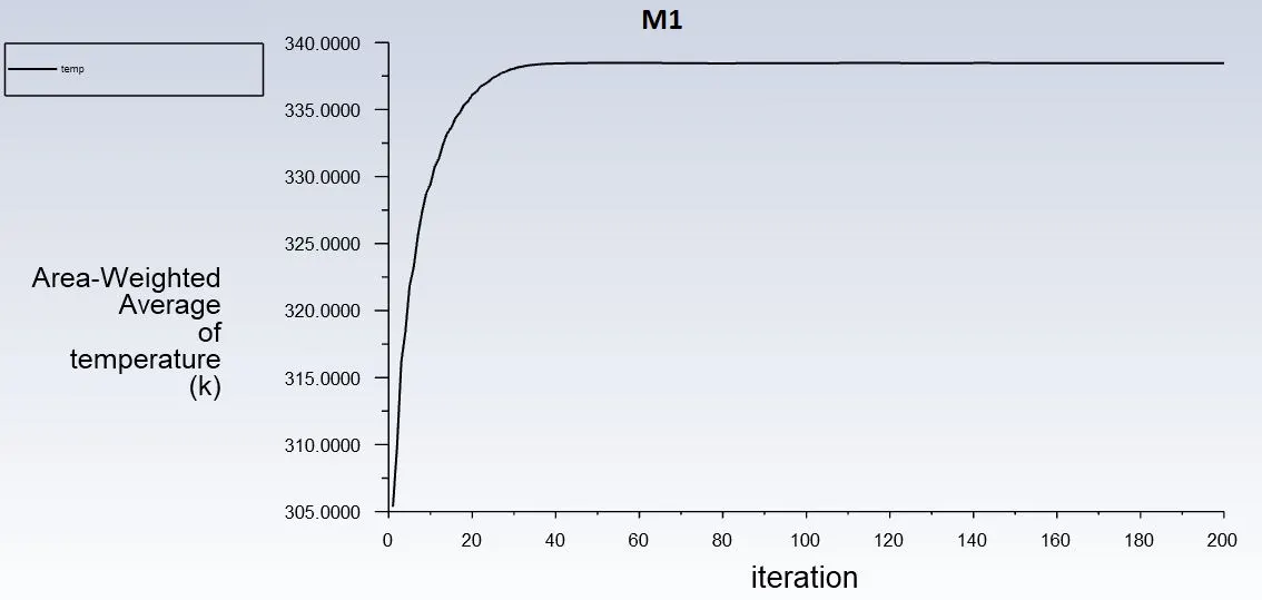
Ø We can see from the above plot that average temperature attained by processor is near 335 to 340 K. So it is near about 64 ⁰C.

Temperature plot on the Plane:

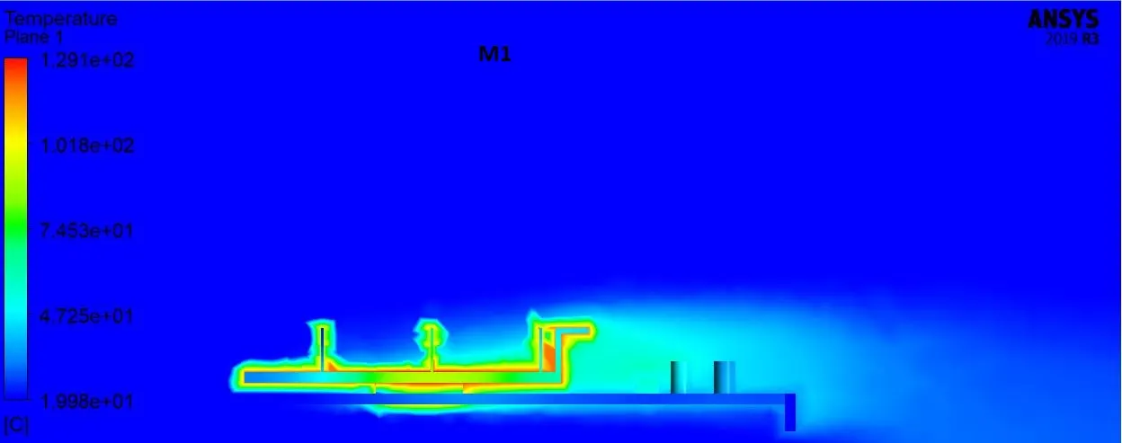
Velocity:

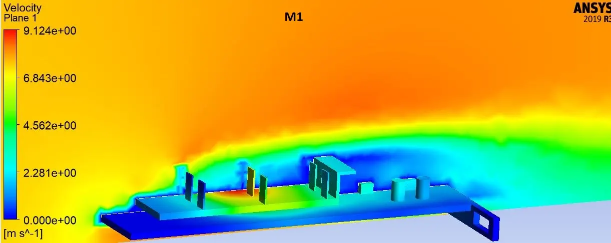
Ø We can see that maximum velocity is about 9.124 m/s.

Ø Low velocity can be observed at the recirculation area behind the fins.

Velocity vectors:

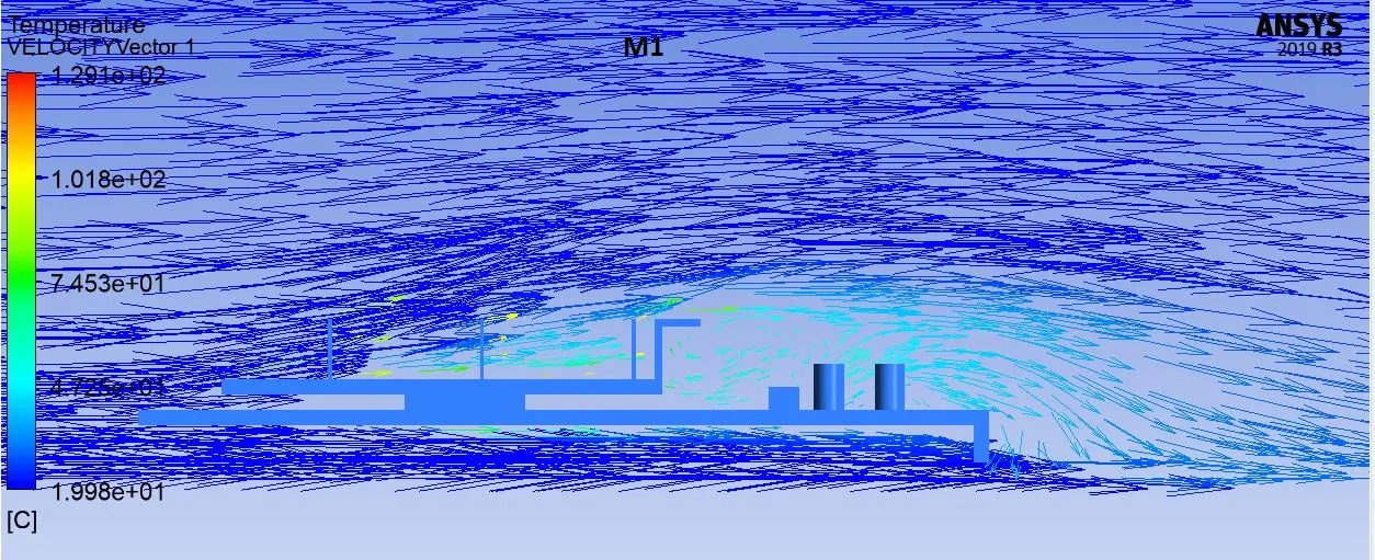
Ø We can see the recirculation of air behind the fins with the vectors.

Velocity plot:

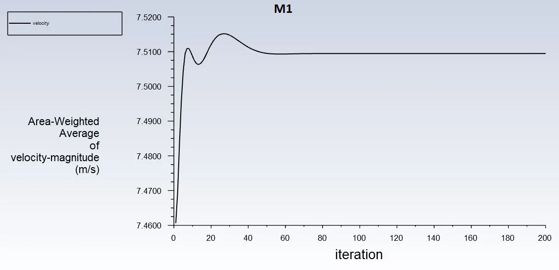
Ø We can see the average velocity is about 7.51 m/s.

Heat Transfer coefficient:

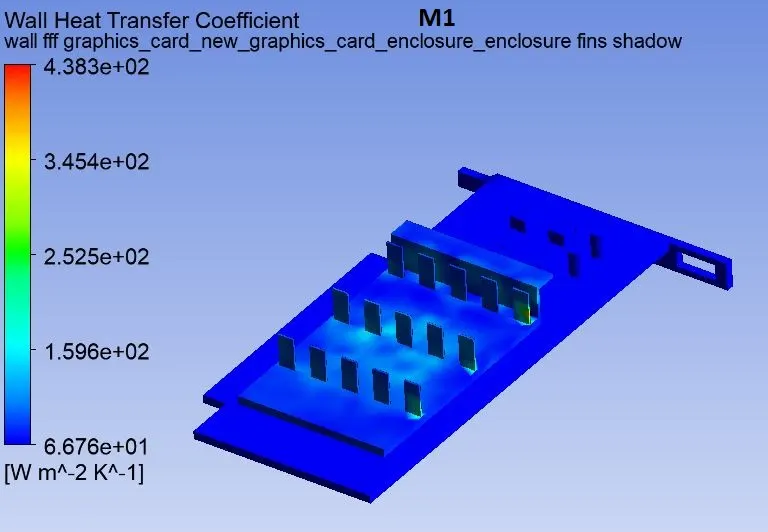
Heat Transfer coefficient (fins):

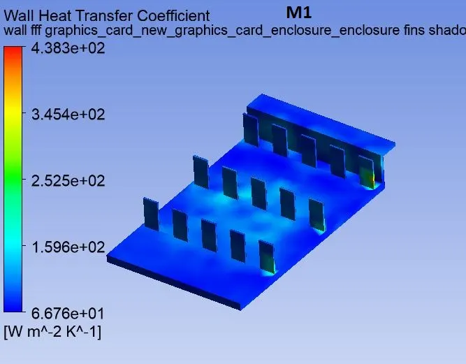
Ø We can see that heat transfer coefficient maximum is 438 W/m²K

Ø IT is measured higher at the fins, as it transfers most heat to the air.

Heat Transfer coefficient on plane:

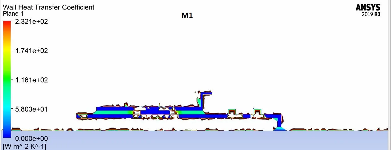
Ø We can see that at the recirculation area behind the fins, where the velocity is lower.

Ø Due to low velocity , lower heat transfer coefficient is observed at that portion.

Hotspot Area:

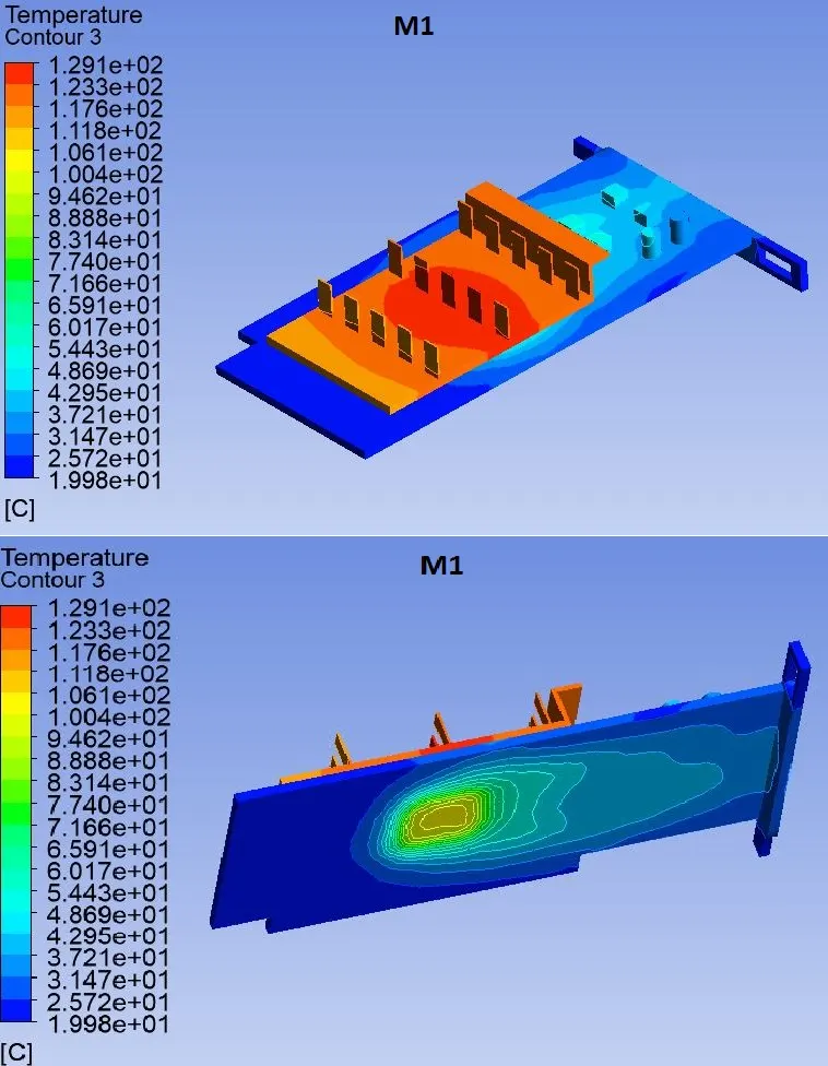
Ø We can see the hotspot at processor on the PCB.

Ø As processor is directly attached to the PCB and the Fins, we can see the high temperature contours near it.

---

Case: M2

Residuals:

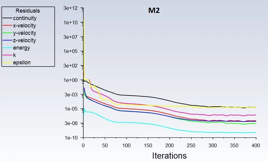
Ø Near about 250, it converges.

Static Temperature:

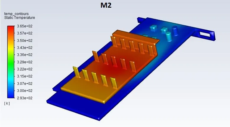
Ø From above plot, 365-293 = 72. So, 273-72=201.

Ø Maximum temperature attained by processor is 201 ⁰C.

Total Temperature:

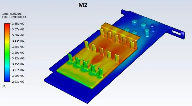
Ø Here also we can observe that front portion of fins is more cooled then rear portion.

Ø Stagnation of air at the rear portion of fins, and so the temperature is high in that area, which can more clearly observed.

Ø Also we can see that at the lower portion of fins are hot, and as we go from lower to upper portion, it can be observed that heat transferred more at the top of the fins.

Ø As air can easily passes on the top of the fins, more it cools, where it is difficult to reach to bottom fast for the air, so it is high in temperature.

Ø Also rear portion of fin, where high temperature can be observed as it collides to the walls of fins, it cools and the rest area remains hotter than that.

Average Temperature:

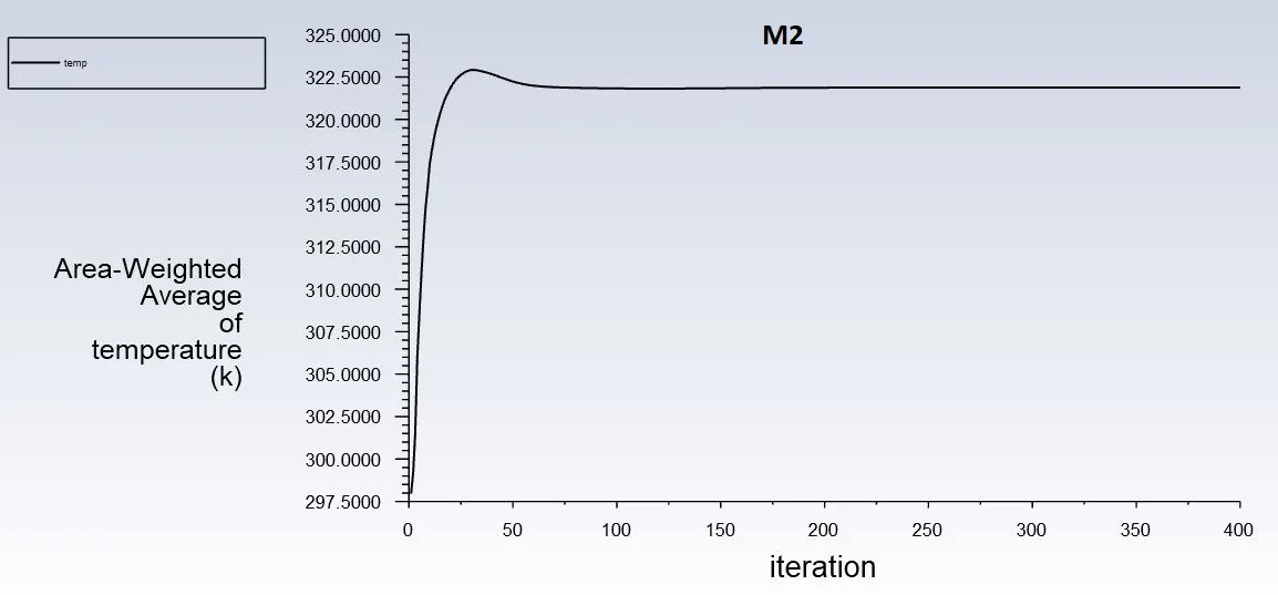
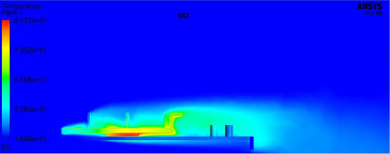
Ø We can see from the above plot that average temperature attained by processor is near 322 K. So it is near about 49 ⁰C.

Temperature plot on the Plane:

Velocity:

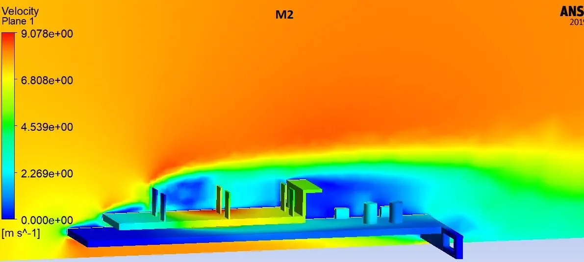
Ø We can see that maximum velocity is about 9 m/s.

Ø Low velocity can be observed at the recirculation area behind the fins.

Velocity vectors:

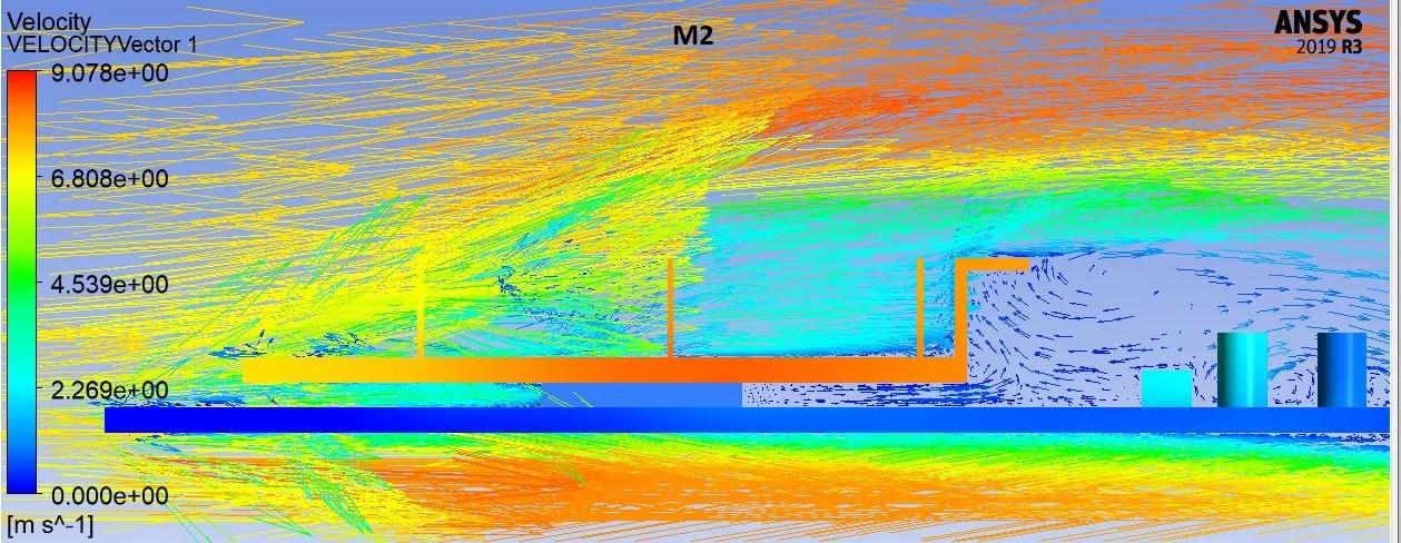
Ø We can see more clearly the recirculation of air behind the fins with the vectors.

Velocity plot:

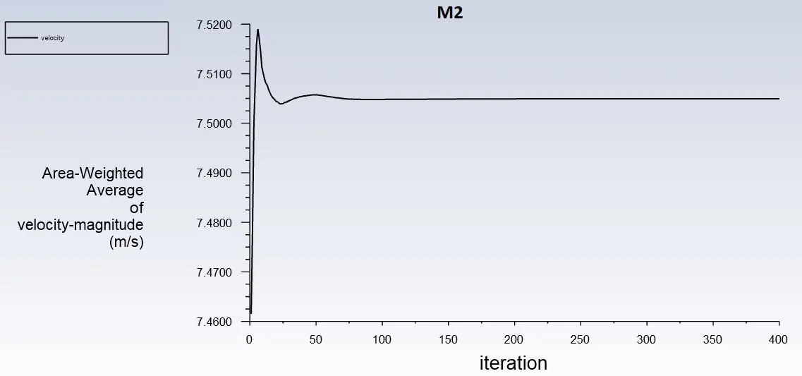
Ø We can see the average velocity is about 7.5 m/s.

Heat Transfer coefficient:

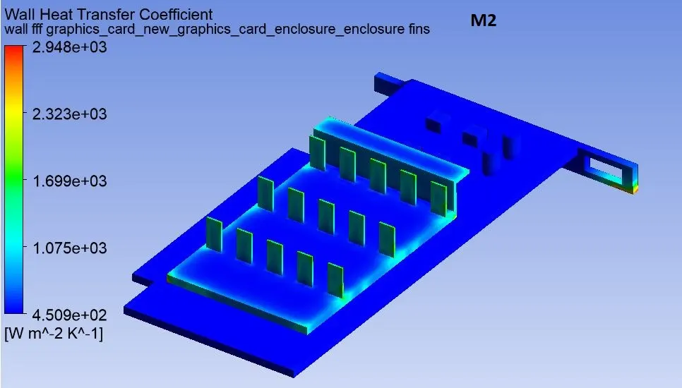
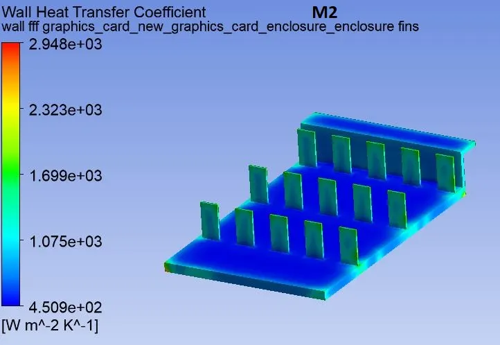
Heat Transfer coefficient (fins):

Ø We can see that heat transfer coefficient maximum is 2948 W/m²K

Ø IT is measured higher at the top of the fins, as it transfers most heat to the air.

Heat Transfer coefficient on plane:

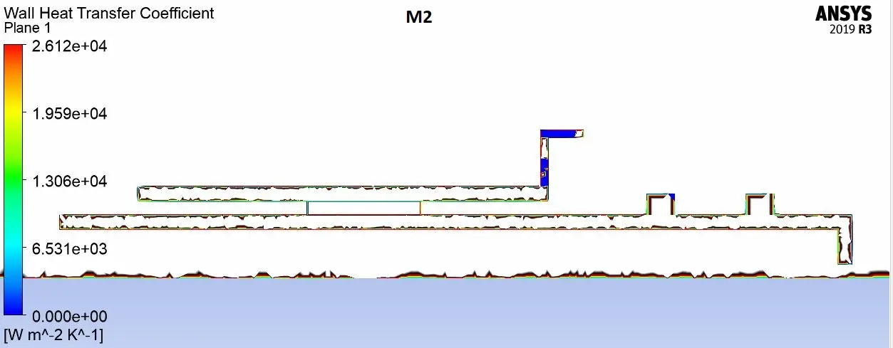
Ø From above image we can see more clearly that lowest heat transfer coefficient measured at rear portion of the fins.

Ø Which is due to low velocity behind the fins or due to recirculation of air

Ø When velocity decreases, Reynolds number decreases, and due to that there can be lower heat transfer coefficient.

Ø Due to fine mesh it is observed very clearly from above image.

Ø Lower the velocity; lower the rate of heat transfer.

Hotspot Area:

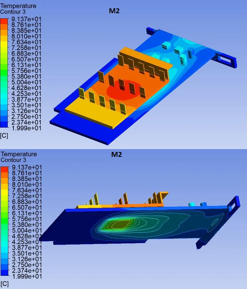
Ø We can see the hotspot at processor on the PCB.

Ø Due to direct attachment of processor to the PCB and the Fins, we can see the high temperature contours near it as discussed in above case.

Observations:

---

Conclusion:

Ø We can conclude from above analysis that conjugate heat transfer gives us results of heat distribution in different components.

Ø We can get clear idea of variations of temperature in different parts attached to the heat source like processors.

Ø Also we can observe that temperature varies as air passes and effect of cooling.

Ø From that we can get maximum temperature attained by the processor and can make changes in its properties as per requirement.

Ø Also we can conclude that Mesh refinement gives us the better and realistic results.

Ø We can see more heat transfer through the convection.

Ø Fins away from inlet are hotter than the fins near the inlet due to direct contact of air neat inlet to the fins area.

Ø Potential hotspot area is near the processor on the PCB and Fins, as they are directly connected to it.

Ø Maximum heat transfer observed at the top of the fins due to direct air contact and lowest heat transfer observed at the recirculation area due to low velocity of air.

Ø Heat transfer coefficient is the quantity, which changes with materials, so its information gives us the idea of improvement for better performance and also important for the design purpose.

Ø Thus CHT study helps to identify hotspots and other coefficients and useful to improve efficiency and performance of the device.

---

References:

1. https://en.wikipedia.org/wiki/Thermal_design_power

2. https://www.howtogeek.com/438898/what-is-tdp-for-cpus-and-gpus/

3. https://www.engineering.com/Hardware/ArticleID/17668/What-Raw-Materials-Are-Used-to-Make-Hardware-in-Computing-Devices.aspx

4. https://en.wikipedia.org/wiki/Video_card

5. https://en.wikipedia.org/wiki/List_of_CPU_power_dissipation_figures

---

Thanks & Regards,

Dharmesh Joshi

---

NOTE: I have attached PDF and WORD file for clarification or for better glance.