Challenge

Project 1

YYogesh Bharti9 Nov 2022

PLEASE FIND THE ATTACHED FILE ALSO.

# Project 1

##Data cleaning & descriptive analytics on Automobile 1985 dataset

import pandas as pd
import numpy as np
import matplotlib.pyplot as plt
import seaborn as sns

df=pd.read_csv("auto_dataset.csv")
print(df)

symboling normalized-losses make aspiration num-of-doors \
0 3 122 alfa-romero std two
1 3 122 alfa-romero std two
2 1 122 alfa-romero std two
3 2 164 audi std four
4 2 164 audi std four
.. ... ... ... ... ...
196 -1 95 volvo std four
197 -1 95 volvo turbo four
198 -1 95 volvo std four
199 -1 95 volvo turbo four
200 -1 95 volvo turbo four

body-style drive-wheels engine-location wheel-base length ... \
0 convertible rwd front 88.6 0.811148 ...
1 convertible rwd front 88.6 0.811148 ...
2 hatchback rwd front 94.5 0.822681 ...
3 sedan fwd front 99.8 0.848630 ...
4 sedan 4wd front 99.4 0.848630 ...
.. ... ... ... ... ... ...
196 sedan rwd front 109.1 0.907256 ...
197 sedan rwd front 109.1 0.907256 ...
198 sedan rwd front 109.1 0.907256 ...
199 sedan rwd front 109.1 0.907256 ...
200 sedan rwd front 109.1 0.907256 ...

compression-ratio horsepower peak-rpm city-mpg highway-mpg price \
0 9.0 111.0 5000.0 21 27 13495.0
1 9.0 111.0 5000.0 21 27 16500.0
2 9.0 154.0 5000.0 19 26 16500.0
3 10.0 102.0 5500.0 24 30 13950.0
4 8.0 115.0 5500.0 18 22 17450.0
.. ... ... ... ... ... ...
196 9.5 114.0 5400.0 23 28 16845.0
197 8.7 160.0 5300.0 19 25 19045.0
198 8.8 134.0 5500.0 18 23 21485.0
199 23.0 106.0 4800.0 26 27 22470.0
200 9.5 114.0 5400.0 19 25 22625.0

city-L/100km horsepower-binned diesel gas
0 11.190476 Medium 0 1
1 11.190476 Medium 0 1
2 12.368421 Medium 0 1
3 9.791667 Medium 0 1
4 13.055556 Medium 0 1
.. ... ... ... ...
196 10.217391 Medium 0 1
197 12.368421 High 0 1
198 13.055556 Medium 0 1
199 9.038462 Medium 1 0
200 12.368421 Medium 0 1

[201 rows x 29 columns]

df.isnull().sum()

symboling 0
normalized-losses 0
make 0
aspiration 0
num-of-doors 0
body-style 0
drive-wheels 0
engine-location 0
wheel-base 0
length 0
width 0
height 0
curb-weight 0
engine-type 0
num-of-cylinders 0
engine-size 0
fuel-system 0
bore 0
stroke 4
compression-ratio 0
horsepower 0
peak-rpm 0
city-mpg 0
highway-mpg 0
price 0
city-L/100km 0
horsepower-binned 1
diesel 0
gas 0

import missingno as ms
plt.title("Missing Values", fontsize=20);
ms.bar(df)

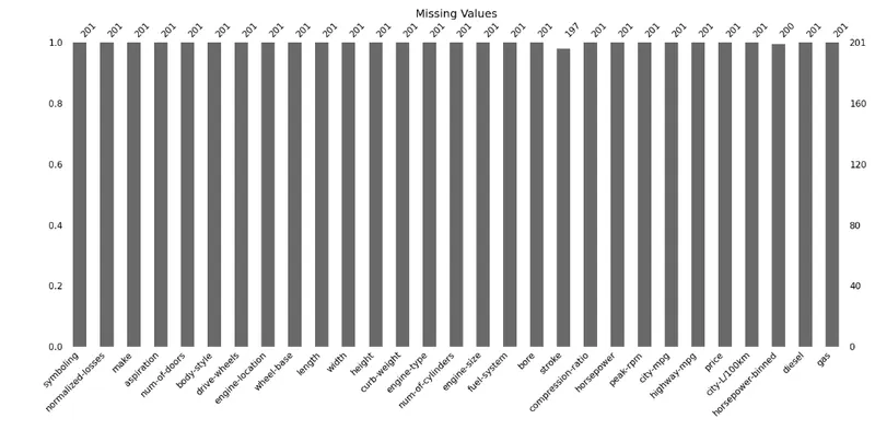
ms.heatmap(df,figsize=(10,8), fontsize=12);
plt.title("Missing Number Correlation Plot");

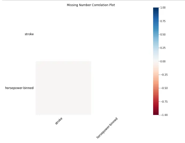
print(df["horsepower-binned"].isnull().sum())
df = df.fillna(0)

df = df.fillna(0)

df.isnull().sum()

symboling 0
normalized-losses 0
make 0
aspiration 0
num-of-doors 0
body-style 0
drive-wheels 0
engine-location 0
wheel-base 0
length 0
width 0
height 0
curb-weight 0
engine-type 0
num-of-cylinders 0
engine-size 0
fuel-system 0
bore 0
stroke 0
compression-ratio 0
horsepower 0
peak-rpm 0
city-mpg 0
highway-mpg 0
price 0
city-L/100km 0
horsepower-binned 0
diesel 0
gas 0

df.info()

RangeIndex: 201 entries, 0 to 200
Data columns (total 29 columns):
# Column Non-Null Count Dtype
--- ------ -------------- -----
0 symboling 201 non-null int64
1 normalized-losses 201 non-null int64
2 make 201 non-null object
3 aspiration 201 non-null object
4 num-of-doors 201 non-null object
5 body-style 201 non-null object
6 drive-wheels 201 non-null object
7 engine-location 201 non-null object
8 wheel-base 201 non-null float64
9 length 201 non-null float64
10 width 201 non-null float64
11 height 201 non-null float64
12 curb-weight 201 non-null int64
13 engine-type 201 non-null object
14 num-of-cylinders 201 non-null object
15 engine-size 201 non-null int64
16 fuel-system 201 non-null object
17 bore 201 non-null float64
18 stroke 201 non-null float64
19 compression-ratio 201 non-null float64
20 horsepower 201 non-null float64
21 peak-rpm 201 non-null float64
22 city-mpg 201 non-null int64
23 highway-mpg 201 non-null int64
24 price 201 non-null float64
25 city-L/100km 201 non-null float64
26 horsepower-binned 201 non-null object
27 diesel 201 non-null int64
28 gas 201 non-null int64
dtypes: float64(11), int64(8), object(10)

df.head(5)

symboling normalized-losses make aspiration num-of-doors body-style drive-wheels engine-location wheel-base length ... compression-ratio horsepower peak-rpm
0 3 122 alfa-romero std two convertible rwd front 88.6 0.811148 ... 9.0 111.0 5000.0 21 27 13495.0 11.190476 Medium 0 1
1 3 122 alfa-romero std two convertible rwd front 88.6 0.811148 ... 9.0 111.0 5000.0 21 27 16500.0 11.190476 Medium 0 1
2 1 122 alfa-romero std two hatchback rwd front 94.5 0.822681 ... 9.0 154.0 5000.0 19 26 16500.0 12.368421 Medium 0 1
3 2 164 audi std four sedan fwd front 99.8 0.848630 ... 10.0 102.0 5500.0 24 30 13950.0 9.791667 Medium 0 1
4 2 164 audi std four sedan 4wd front 99.4 0.848630 ... 8.0 115.0 5500.0 18 22 17450.0 13.055556 Medium 0 1

df.tail(5)

symboling normalized-losses make aspiration num-of-doors body-style drive-wheels engine-location wheel-base length ... compression-ratio horsepower
196 -1 95 volvo std four sedan rwd front 109.1 0.907256 ... 9.5 114.0 5400.0 23 28 16845.0 10.217391 Medium 0 1
197 -1 95 volvo turbo four sedan rwd front 109.1 0.907256 ... 8.7 160.0 5300.0 19 25 19045.0 12.368421 High 0 1
198 -1 95 volvo std four sedan rwd front 109.1 0.907256 ... 8.8 134.0 5500.0 18 23 21485.0 13.055556 Medium 0 1
199 -1 95 volvo turbo four sedan rwd front 109.1 0.907256 ... 23.0 106.0 4800.0 26 27 22470.0 9.038462 Medium 1 0
200 -1 95 volvo turbo four sedan rwd front 109.1 0.907256 ... 9.5 114.0 5400.0 19 25 22625.0 12.368421 Medium 0 1

df.columns
Index(['symboling', 'normalized-losses', 'make', 'aspiration', 'num-of-doors',
'body-style', 'drive-wheels', 'engine-location', 'wheel-base', 'length',
'width', 'height', 'curb-weight', 'engine-type', 'num-of-cylinders',
'engine-size', 'fuel-system', 'bore', 'stroke', 'compression-ratio',
'horsepower', 'peak-rpm', 'city-mpg', 'highway-mpg', 'price',
'city-L/100km', 'horsepower-binned', 'diesel', 'gas']

df.info()

RangeIndex: 201 entries, 0 to 200
Data columns (total 29 columns):
# Column Non-Null Count Dtype
--- ------ -------------- -----
0 symboling 201 non-null int64
1 normalized-losses 201 non-null int64
2 make 201 non-null object
3 aspiration 201 non-null object
4 num-of-doors 201 non-null object
5 body-style 201 non-null object
6 drive-wheels 201 non-null object
7 engine-location 201 non-null object
8 wheel-base 201 non-null float64
9 length 201 non-null float64
10 width 201 non-null float64
11 height 201 non-null float64
12 curb-weight 201 non-null int64
13 engine-type 201 non-null object
14 num-of-cylinders 201 non-null object
15 engine-size 201 non-null int64
16 fuel-system 201 non-null object
17 bore 201 non-null float64
18 stroke 201 non-null float64
19 compression-ratio 201 non-null float64
20 horsepower 201 non-null float64
21 peak-rpm 201 non-null float64
22 city-mpg 201 non-null int64
23 highway-mpg 201 non-null int64
24 price 201 non-null float64
25 city-L/100km 201 non-null float64
26 horsepower-binned 201 non-null object
27 diesel 201 non-null int64
28 gas 201 non-null int64

symboling 0.840796
normalized-losses 122.000000
horsepower 103.405534
stroke 3.192090
wheel-base 98.797015
engine-size 126.875622
bore 3.330692
stroke 3.192090
compression-ratio 10.164279
horsepower 103.405534
peak-rpm 5117.665368
city-mpg 25.179104
highway-mpg 30.686567
price 13207.129353
city-L/100km 9.944145
diesel 0.099502
gas 0.900498

symboling 3
normalized-losses 256
horsepower 262.0
stroke 4.17
wheel-base 120.9
engine-size 326
fuel-system spfi
bore 3.94
stroke 4.17
compression-ratio 23.0
horsepower 262.0
peak-rpm 6600.0
city-mpg 49
highway-mpg 54
price 45400.0
city-L/100km 18.076923
diesel 1
gas 1

df[["symboling","normalized-losses","horsepower","stroke",'wheel-base', 'length',
'width', 'height', 'curb-weight','engine-size', 'fuel-system', 'bore', 'stroke', 'compression-ratio',
'horsepower', 'peak-rpm', 'city-mpg', 'highway-mpg', 'price',
'city-L/100km', 'diesel', 'gas']].median()
symboling 1.000000
normalized-losses 122.000000
horsepower 95.000000
stroke 3.290000
wheel-base 97.000000
length 0.832292
width 0.909722
height 54.100000
curb-weight 2414.000000
engine-size 120.000000
bore 3.310000
stroke 3.290000
compression-ratio 9.000000
horsepower 95.000000
peak-rpm 5125.369458
city-mpg 24.000000
highway-mpg 30.000000
price 10295.000000
city-L/100km 9.791667
diesel 0.000000
gas 1.000000

df[["symboling","normalized-losses","horsepower","stroke",'wheel-base',
'engine-size', 'fuel-system', 'bore', 'stroke', 'compression-ratio',
'horsepower', 'peak-rpm', 'city-mpg', 'highway-mpg', 'price',
'city-L/100km', 'diesel', 'gas']].min()
symboling -2
normalized-losses 65
horsepower 48.0
stroke 0.0
wheel-base 86.6
engine-size 61
fuel-system 1bbl
bore 2.54
stroke 0.0
compression-ratio 7.0
horsepower 48.0
peak-rpm 4150.0
city-mpg 13
highway-mpg 16
price 5118.0
city-L/100km 4.795918
diesel 0
gas 0

symboling 1.254802
normalized-losses 31.996250
horsepower 37.365700
stroke 0.554809
wheel-base 6.066366
engine-size 41.546834
bore 0.268072
stroke 0.554809
compression-ratio 4.004965
horsepower 37.365700
peak-rpm 478.113805
city-mpg 6.423220
highway-mpg 6.815150
price 7947.066342
city-L/100km 2.534599
diesel 0.300083
gas 0.300083

import statistics as st
print(st.median_low(df['price']))
print(st.median_low(df['normalized-losses']))
print(st.median_low(df['horsepower']))
print(st.median_low(df['engine-size']))
print(st.median_low(df['peak-rpm']))
print(st.median_low(df['city-mpg']))
print(st.median_low(df['city-L/100km']))

10295.0
122
95.0
120
5125.369458128079
24
9.791666666666666

print(st.median_high(df['price']))
print(st.median_high(df['normalized-losses']))
print(st.median_high(df['horsepower']))
print(st.median_high(df['engine-size']))
print(st.median_high(df['peak-rpm']))
print(st.median_high(df['city-mpg']))
print(st.median_high(df['city-L/100km']))

10295.0
122
95.0
120
5125.369458128079
24
9.791666666666666

variance()
This returns the variance of the sample.
This is the second moment about the mean and a larger value denotes a rather spread-out set of data.
You can use this when your data is a sample out of a population.

print(st.variance(df['price']))
print(st.variance(df['normalized-losses']))
print(st.variance(df['horsepower']))
print(st.variance(df['engine-size']))
print(st.variance(df['peak-rpm']))
print(st.variance(df['city-mpg']))
print(st.variance(df['city-L/100km']))

62841655.16734734
1018.6666666666666
1389.2492530166392
1717.5516942649933
227455.53288605926
41.05249870052722
6.392232253809319

pvariance()
This returns the population variance of data.
Use this to calculate variance from an entire population.

print(st.pvariance(df['price']))
print(st.pvariance(df['normalized-losses']))
print(st.pvariance(df['horsepower']))
print(st.pvariance(df['engine-size']))
print(st.pvariance(df['peak-rpm']))
print(st.pvariance(df['city-mpg']))
print(st.pvariance(df['city-L/100km']))

stdev()
This returns the standard deviation for the sample. This is equal to the square root of the sample variance.

print(st.stdev(df['price']))
print(st.stdev(df['normalized-losses']))
print(st.stdev(df['horsepower']))
print(st.stdev(df['engine-size']))
print(st.stdev(df['peak-rpm']))
print(st.stdev(df['city-mpg']))
print(st.stdev(df['city-L/100km']))

62841655.16734734
1018.6666666666666
1389.2492530166392
1717.5516942649933
227455.53288605926
41.05249870052722
6.392232253809319

pstdev()
This returns the population standard deviation. This is the square root of population variance.

print(st.pstdev(df['price']))
print(st.pstdev(df['normalized-losses']))
print(st.pstdev(df['horsepower']))
print(st.pstdev(df['engine-size']))
print(st.pstdev(df['peak-rpm']))
print(st.pstdev(df['city-mpg']))
print(st.pstdev(df['city-L/100km']))

7927.272870751161
31.91655787622886
37.27263410354357
41.4433552486402
476.92298422917224
6.4072223857555635
2.5282864263784117

skew

df.skew()

symboling 0.197370
normalized-losses 0.846546
wheel-base 1.031261
length 0.154446
width 0.875029
height 0.029173
curb-weight 0.705804
engine-size 1.979144
bore -0.032730
stroke -3.860477
compression-ratio 2.584462
horsepower 1.146517
peak-rpm 0.107770
city-mpg 0.680433
highway-mpg 0.549507
price 1.809675
city-L/100km 0.592383
diesel 2.696072
gas -2.696072

df.describe()
symboling normalized-losses wheel-base length width height curb-weight engine-size bore stroke compression-ratio horsepower peak-rpm city-mpg highway-mpg price city-L/100km diesel gas
count 201.000000 201.00000 201.000000 201.000000 201.000000 201.000000 201.000000 201.000000 201.000000 201.000000 201.000000 201.000000 201.000000 201.000000 201.000000 201.000000 201.000000 201.000000 201.000000
mean 0.840796 122.00000 98.797015 0.837102 0.915126 53.766667 2555.666667 126.875622 3.330692 3.192090 10.164279 103.405534 5117.665368 25.179104 30.686567 13207.129353 9.944145 0.099502 0.900498
std 1.254802 31.99625 6.066366 0.059213 0.029187 2.447822 517.296727 41.546834 0.268072 0.554809 4.004965 37.365700 478.113805 6.423220 6.815150 7947.066342 2.534599 0.300083 0.300083
min -2.000000 65.00000 86.600000 0.678039 0.837500 47.800000 1488.000000 61.000000 2.540000 0.000000 7.000000 48.000000 4150.000000 13.000000 16.000000 5118.000000 4.795918 0.000000 0.000000
25% 0.000000 101.00000 94.500000 0.801538 0.890278 52.000000 2169.000000 98.000000 3.150000 3.100000 8.600000 70.000000 4800.000000 19.000000 25.000000 7775.000000 7.833333 0.000000 1.000000
50% 1.000000 122.00000 97.000000 0.832292 0.909722 54.100000 2414.000000 120.000000 3.310000 3.290000 9.000000 95.000000 5125.369458 24.000000 30.000000 10295.000000 9.791667 0.000000 1.000000
75% 2.000000 137.00000 102.400000 0.881788 0.925000 55.500000 2926.000000 141.000000 3.580000 3.410000 9.400000 116.000000 5500.000000 30.000000 34.000000 16500.000000 12.368421 0.000000 1.000000
max 3.000000 256.00000 120.900000 1.000000 1.000000 59.800000 4066.000000 326.000000 3.940000 4.170000 23.000000 262.000000 6600.000000 49.000000 54.000000 45400.000000 18.076923 1.000000 1.000000

print(df.describe(include=['object']))
make aspiration num-of-doors body-style drive-wheels \
count 201 201 201 201 201
unique 22 2 2 5 3
top toyota std four sedan fwd
freq 32 165 115 94 118

engine-location engine-type num-of-cylinders fuel-system \
count 201 201 201 201
unique 2 6 7 8
top front ohc four mpfi
freq 198 145 157 92

horsepower-binned
count 201
unique 4
top Low
freq 115

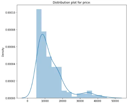
plt.figure(figsize=(8,7))
sns.distplot(df['price'])
plt.title("Distribution plot for price:")

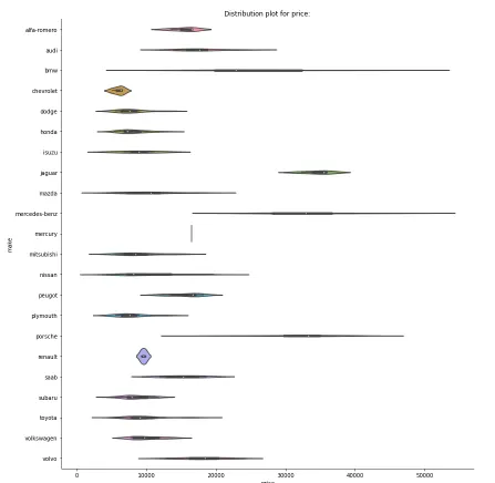
sns.catplot(x="price", y="make",
kind="violin", data=df, height=12);
plt.title("Distribution plot for price:")

plt.figure(figsize=(8,7))
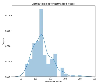
sns.distplot(df['normalized-losses'])
plt.title("Distribution plot for normalized-losses:")

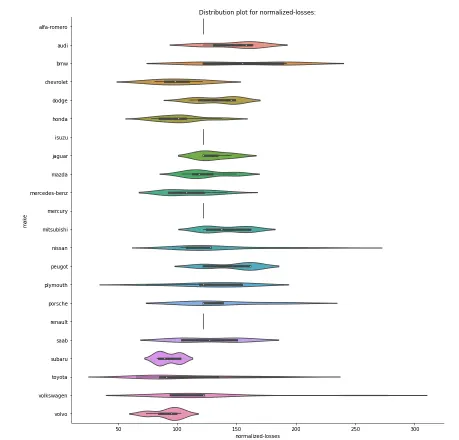
sns.catplot(x="normalized-losses", y="make",
kind="violin", data=df, height=12);
plt.title("Distribution plot for normalized-losses:")

plt.figure(figsize=(8,7))
sns.distplot(df['curb-weight'])
plt.title("Distribution plot for curb-weight:")

sns.catplot(x="curb-weight", y="make",
kind="violin", data=df, height=12);
plt.title("Distribution plot for curb-weight:")

plt.figure(figsize=(8,7))
sns.distplot(df['engine-size'])
plt.title("Distribution plot for engine-size:")

sns.catplot(x="engine-size", y="make",
kind="violin", data=df, height=12);
plt.title("Distribution plot for engine-size:")

plt.figure(figsize=(8,7))
sns.distplot(df['compression-ratio'])
plt.title("Distribution plot for compression-ratio:")
sns.catplot(x="compression-ratio", y="make",
kind="violin", data=df, height=12);
plt.title("Distribution plot for compression-ratio:")

plt.figure(figsize=(8,7))
sns.distplot(df['horsepower'])
plt.title("Distribution plot for horsepower:")

sns.catplot(x="horsepower", y="make",
kind="violin", data=df, height=12);
plt.title("Distribution plot for horsepower:")

plt.figure(figsize=(8,7))
sns.distplot(df['peak-rpm'])
plt.title("Distribution plot for peak-rpm:")

sns.catplot(x="peak-rpm", y="make",
kind="violin", data=df, height=12);
plt.title("Distribution plot for peak-rpm:")

plt.figure(figsize=(8,7))
sns.distplot(df['city-mpg'])
plt.title("Distribution plot for city-mpg:")

sns.catplot(x="city-mpg", y="make",
kind="violin", data=df, height=12);
plt.title("Distribution plot for price:")

plt.figure(figsize=(8,7))
sns.distplot(df['city-L/100km'])
plt.title("Distribution plot for city-L/100km :")

sns.catplot(x="city-L/100km", y="make",
kind="violin", data=df, height=12);
plt.title("Distribution plot for city-L/100km:")

plt.figure(figsize=(8,7))
sns.distplot(df['diesel'])
plt.title("Distribution plot for diesel:")

sns.catplot(x="diesel", y="make",
kind="violin", data=df, height=12);
plt.title("Distribution plot for diesel:")

plt.figure(figsize=(8,7))
sns.distplot(df['gas'])
plt.title("Distribution plot for gas:")

sns.catplot(x="gas", y="make",
kind="violin", data=df, height=12);
plt.title("Distribution plot for gas:")

plt.figure(figsize=(15,7))
sns.boxplot(x = "price", data = df, showmeans=True)
plt.title("Boxplot for Price")
plt.show()

plt.figure(figsize=(15,7))
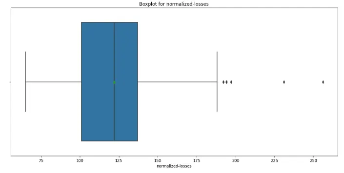
sns.boxplot(x = "normalized-losses", data = df, showmeans=True)
plt.title("Boxplot for normalized-losses")
plt.show()

plt.figure(figsize=(15,7))
sns.boxplot(x = "curb-weight", data = df, showmeans=True)
plt.title("Boxplot for curb-weight")
plt.show()

plt.figure(figsize=(15,7))
sns.boxplot(x = "engine-size", data = df, showmeans=True)
plt.title("Boxplot for engine-size")
plt.show()

plt.figure(figsize=(15,7))
sns.boxplot(x = "horsepower", data = df, showmeans=True)
plt.title("Boxplot for horsepower")
plt.show()

plt.figure(figsize=(15,7))
sns.boxplot(x = "compression-ratio", data = df, showmeans=True)
plt.title("Boxplot for compression-ratio")
plt.show()

plt.figure(figsize=(15,7))
sns.boxplot(x = "city-mpg", data = df, showmeans=True)
plt.title("Boxplot for city-mpg")
plt.show()

plt.figure(figsize=(15,7))
sns.boxplot(x = "city-L/100km", data = df, showmeans=True)
plt.title("Boxplot for city-L/100km")
plt.show()

plt.figure(figsize=(15,7))
sns.boxplot(x = "diesel", data = df, showmeans=True)
plt.title("Boxplot for diesel")
plt.show()

plt.figure(figsize=(15,7))
sns.boxplot(x = "gas", data = df, showmeans=True)
plt.title("Boxplot for gas")
plt.show()

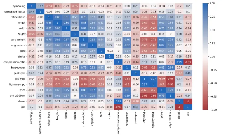
correlation = df.corr().round(2) # creating a 2-D Matrix with correlation plots
correlation
plt.figure(figsize = (15,8))
sns.heatmap(correlation, annot=True, cmap='vlag_r', vmin=-1, vmax=1)

plt.figure(figsize=(7,5))
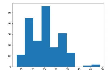
plt.hist(df["city-mpg"])

(array([11., 45., 24., 56., 18., 31., 13., 0., 1., 2.]),
array([13. , 16.6, 20.2, 23.8, 27.4, 31. , 34.6, 38.2, 41.8, 45.4, 49. ])

pair=df[["horsepower","price","normalized-losses","engine-size","peak-rpm","city-mpg","highway-mpg","wheel-base","city-L/100km","make","aspiration","num-of-doors","body-style","engine-type"]]

print(df["aspiration"].unique())
print(df["num-of-doors"].unique())
print(df["body-style"].unique())
print(df["engine-type"].unique())
print(df["make"].unique())
print(df["horsepower-binned"].unique())

['std' 'turbo']
['two' 'four']
['convertible' 'hatchback' 'sedan' 'wagon' 'hardtop']
['dohc' 'ohcv' 'ohc' 'l' 'rotor' 'ohcf']
['alfa-romero' 'audi' 'bmw' 'chevrolet' 'dodge' 'honda' 'isuzu' 'jaguar'
'mazda' 'mercedes-benz' 'mercury' 'mitsubishi' 'nissan' 'peugot'
'plymouth' 'porsche' 'renault' 'saab' 'subaru' 'toyota' 'volkswagen'
'volvo']
['Medium' 'Low' 'High' 0]

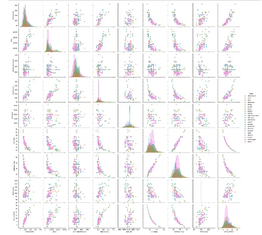
sns.pairplot(pair, hue ='make')
plt.show()

sns.pairplot(pair, hue ='aspiration')
plt.show()

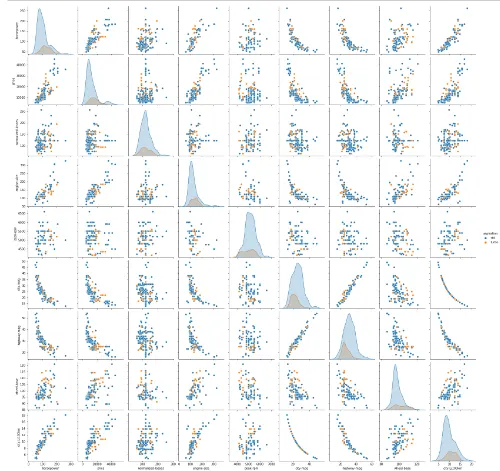
sns.pairplot(pair, hue ="num-of-doors")
plt.show()

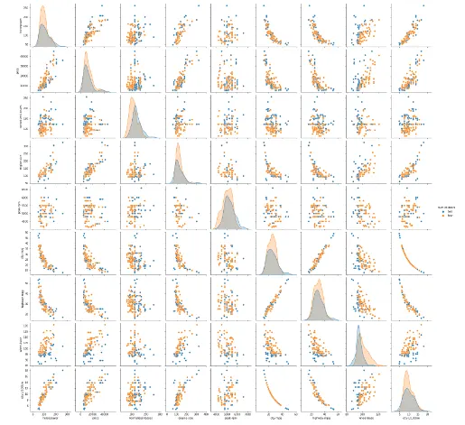
sns.pairplot(pair, hue ="engine-type")
plt.show()

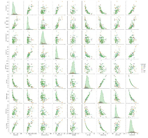
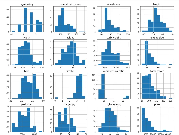
df.hist(figsize=(15,15))
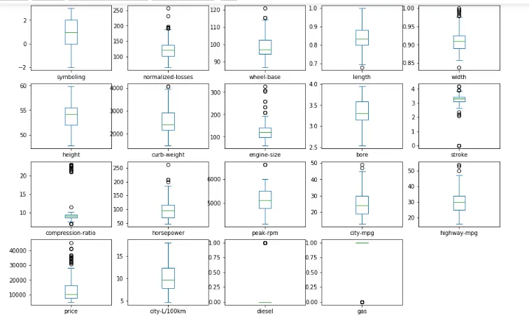
df.plot(kind='box',layout=(6,5),subplots=True,sharex=False,sharey=False,figsize=(15,15))

symboling AxesSubplot(0.125,0.772143;0.133621x0.107857)
normalized-losses AxesSubplot(0.285345,0.772143;0.133621x0.107857)
wheel-base AxesSubplot(0.44569,0.772143;0.133621x0.107857)
length AxesSubplot(0.606034,0.772143;0.133621x0.107857)
width AxesSubplot(0.766379,0.772143;0.133621x0.107857)
height AxesSubplot(0.125,0.642714;0.133621x0.107857)
curb-weight AxesSubplot(0.285345,0.642714;0.133621x0.107857)
engine-size AxesSubplot(0.44569,0.642714;0.133621x0.107857)
bore AxesSubplot(0.606034,0.642714;0.133621x0.107857)
stroke AxesSubplot(0.766379,0.642714;0.133621x0.107857)
compression-ratio AxesSubplot(0.125,0.513286;0.133621x0.107857)
horsepower AxesSubplot(0.285345,0.513286;0.133621x0.107857)
peak-rpm AxesSubplot(0.44569,0.513286;0.133621x0.107857)
city-mpg AxesSubplot(0.606034,0.513286;0.133621x0.107857)
highway-mpg AxesSubplot(0.766379,0.513286;0.133621x0.107857)
price AxesSubplot(0.125,0.383857;0.133621x0.107857)
city-L/100km AxesSubplot(0.285345,0.383857;0.133621x0.107857)
diesel AxesSubplot(0.44569,0.383857;0.133621x0.107857)
gas AxesSubplot(0.606034,0.383857;0.133621x0.107857)

Project 1

Ship work like this
in your own course.

Talk to a career counsellor

Ship work like thisin your own course.

Talk to a career counsellor

Ship work like this
in your own course.