Project 1

Objective: Data cleaning on Automobile 1985 dataset and perform descriptive analytics

# Data cleaning of a Automobile dataset

#importing packages
import pandas as pd
import numpy as np
import seaborn as sns

import matplotlib.mlab as mlab
import matplotlib
import matplotlib.pyplot as plt

#read the data
df = pd.read_csv('D:/MLnAI/Challenges/Project1/auto.csv')
print(df.head())
print(df.info()) 
print(df.describe(include="all")) # includes variable type 'object'

Sample of raw automobile dataset

Information on dataset

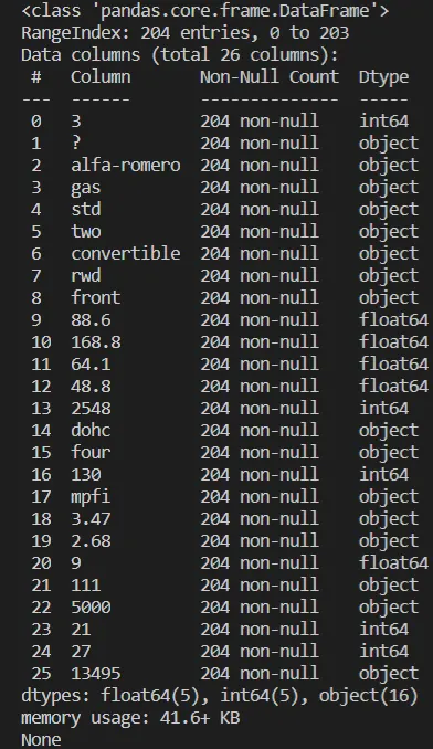
Description of dataset

# Adding column names to dataframe
df.columns = ["symboling", "normalized-losses", "make", "fuel", "aspiration", "number of doors", "body-style", "drive-wheels", "engine-location",
"wheel-base","length", "width", "height", "curb-weight", "engine-type", "num-of-cylinders", "engine-size", "fuel-system", "bore",
"stroke", "compression-ratio", "horsepower", "peak-rpm", "city-mpg", "highway-mpg", "price"]

#Display the column names
print(list(df.columns))
print(df.head())
print(df.describe())

Column headings added to the dataset

Dataset with new column headers

Sample of dataset :

The sign "?" has to be replaced and is replaced with NaN

df = df.replace('?', np.NAN)
print(df.head())

Sample of refined dataset

print(df.loc[7:12,['price']])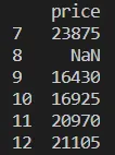

The NaN value present in the column "price" will be replaced by the mean of the column "price". This opeartion will be followed in other columns were NaN value are present.

df[["price"]]=df[["price"]].astype(str).astype(float)
mean = df[["price"]].mean(axis=0, skipna= True)
#print('mean value is: ',mean)
df[["price"]] = df[["price"]].replace(np.NaN, mean)

df[["normalized-losses"]]=df[["normalized-losses"]].astype(str).astype(float)  # Convert column from object to float to relace NAN with mean value
mean = df[["normalized-losses"]].mean(axis=0, skipna= True)
#print('mean value is: ',mean)
df[["normalized-losses"]] = df[["normalized-losses"]].replace(np.NaN, mean)

df[["bore"]]=df[["bore"]].astype(str).astype(float)
mean = df[["bore"]].mean(axis=0, skipna= True)
#print('mean value is: ',mean)
df[["bore"]] = df[["bore"]].replace(np.NaN, mean)

df[["stroke"]]=df[["stroke"]].astype(str).astype(float)
mean = df[["stroke"]].mean(axis=0, skipna= True)
#print('mean value is: ',mean)
df[["stroke"]] = df[["stroke"]].replace(np.NaN, mean)

df[["horsepower"]]=df[["horsepower"]].astype(str).astype(float)
mean = df[["horsepower"]].mean(axis=0, skipna= True)
#print('mean value is: ',mean)
df[["horsepower"]] = df[["horsepower"]].replace(np.NaN, mean)
print(df.loc[129:134,['horsepower']])

df[["peak-rpm"]]=df[["peak-rpm"]].astype(str).astype(float)
mean = df[["peak-rpm"]].mean(axis=0, skipna= True)
#print('mean value is: ',mean)
df[["peak-rpm"]] = df[["peak-rpm"]].replace(np.NaN, mean)

print(df.info())
#print(df)
print(df.loc[7:12,['price']])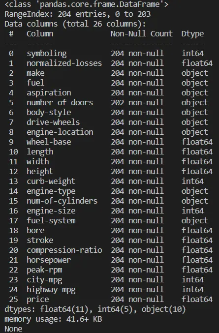

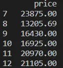
Binning the data

# Binning the price to low, medium, High
binwidth = int((max(df['price'])-min(df['price']))/3.0)
bins = range(int(min(df['price'])),int(max(df['price'])),binwidth)
df['price-binned'] = pd.cut(df['price'],bins, labels=['Low','Medium', 'High'])
#df["Price_Bin"] = df['price-binned']
#print(df.loc[15:20,['price','price-binned']])
print(df)

# Binning the horsepower to low, medium, High
binwidth = int((max(df['horsepower'])-min(df['horsepower']))/3.0)
bins = range(int(min(df['horsepower'])),int(max(df['horsepower'])),binwidth)
df['horsepower-binned'] = pd.cut(df['horsepower'],bins, labels=['Low','Medium', 'High'])
#print(df.loc[1:20,['horsepower','horsepower-binned']])
#print(df.info())
print(df)

# label encoding the data 
from sklearn.preprocessing import LabelEncoder 
le = LabelEncoder() 
df['make-binned']= le.fit_transform(df['make']) 
print(df['make-binned'])
print(df)

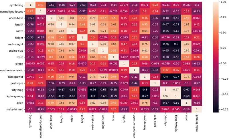
# Visualization of correlation with seaborn heatmap
f,ax = plt.subplots(figsize = (10,10))
sns.heatmap(df.corr(),annot = True)
plt.show()

Coorelation map

# Numerical variables and their correlation with price
sns.regplot(x="engine-size", y="price", data=df)
plt.show()
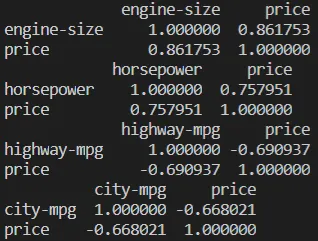
print(df[["engine-size", "price"]].corr())
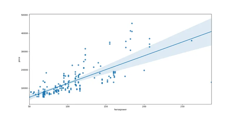
sns.regplot(x="horsepower", y="price", data=df)
plt.show()
print(df[["horsepower", "price"]].corr())
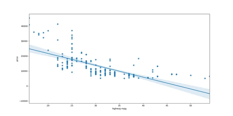
sns.regplot(x="highway-mpg", y="price", data=df)
plt.show()
print(df[["highway-mpg", "price"]].corr())
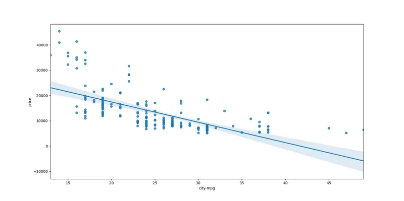
sns.regplot(x="city-mpg", y="price", data=df)
plt.show()
print(df[["city-mpg", "price"]].corr())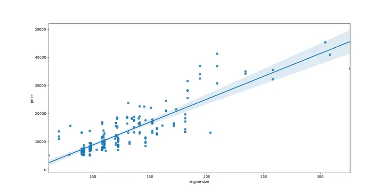

# Categorical variables and their correlation with price

sns.boxplot(x="engine-location", y="price", data=df)
plt.show()
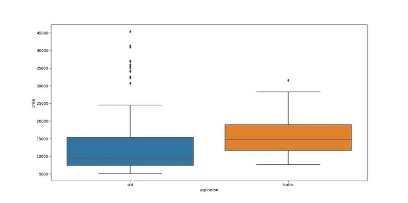
sns.boxplot(x="aspiration", y="price", data=df)
plt.show()
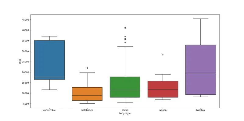
sns.boxplot(x="body-style", y="price", data=df)
plt.show()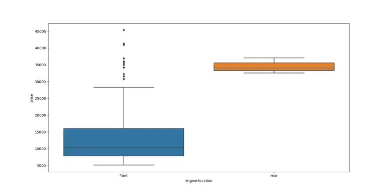

The data is now cleaned and well described.