Project 1

Aim:

To perform data cleaning and descriptive analytics on the Automobile 1985 dataset

Dataset:

The dataset is about cars from 1985, It consists of:

Number of rows: 201

Number of columns: 29

Data Cleaning:

• The dataset is read using pandas library
• The info of the dataset are

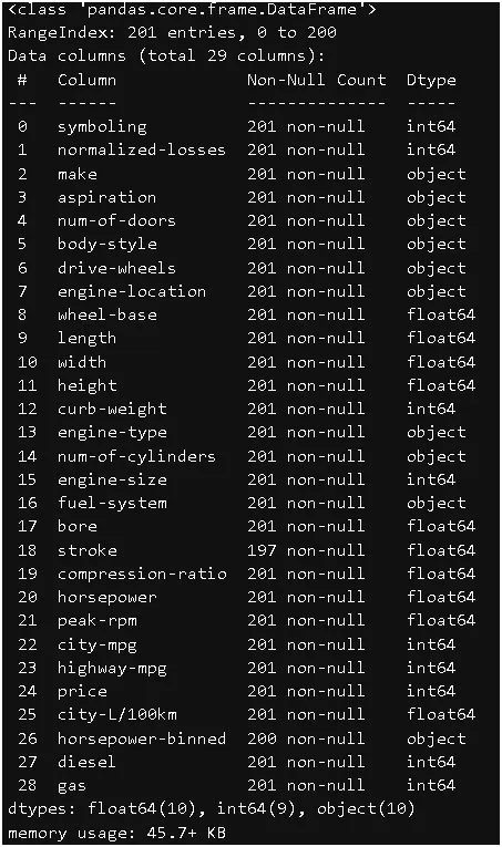
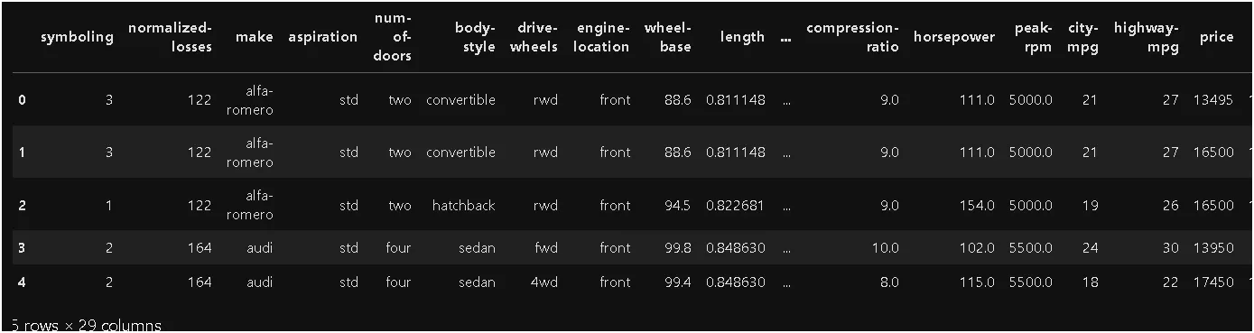
• The first 5 records of the dataset

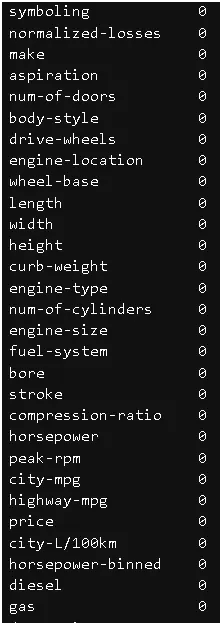
• filled the missing values

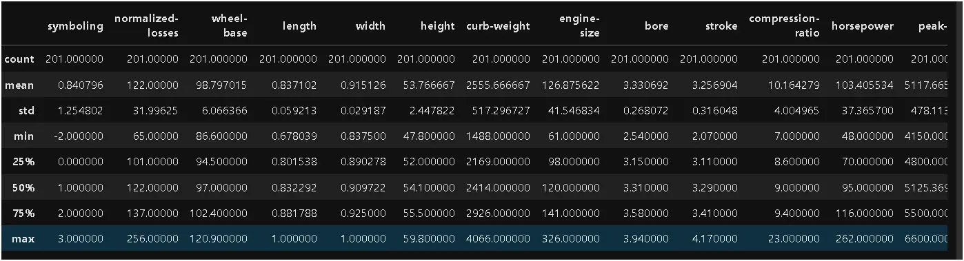
• To see the mean, standard deviation, max, etc of dataset

Descriptive Summary:
Summary Statistics for these include:

• Average price: $13,207
• Average horsepower: 103.4
• Average City mileage (city-mpg): 25.17 mpg
• Average Highway mileage: 30.69 mpg
• Average city-L/100km: 9.9 L/100 km

Price Distribution:

• The average price of vehicles in the dataset is around 13,207(dollers) with a wide range from 5,118(dollers) to $45,400. This indicates that the dataset likely contains a mix of both budget and luxury vehicles.

Horsepower:

• The horsepower feature shows an average value of 103.4 HP, with a maximum of 262 HP. This suggests that the dataset contains vehicles of varying performance levels.

Fuel Economy:

• The city-mpg feature shows that vehicles have an average of around 25 miles per gallon (mpg) in the city, with the maximum reaching 49 mpg.

We plot a correlation matrix to find highly correlated features

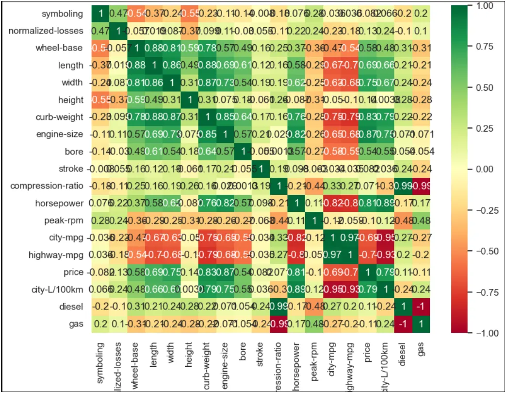
Using standard scaler the whole data set is standardized

code:

# importing libraries

import pandas as pd

from sklearn.preprocessing import StandardScaler, LabelEncoder

import matplotlib.pyplot as plt

import seaborn as sns

# Load the data

data = pd.read_csv('auto_clean.csv')

# Display the first few rows to understand the structure of the dataset

data.head()

# Info about data

data.info()

# checking missing Values

data.isna().sum()

# filling missing values

data['stroke'] = data['stroke'].fillna(data['stroke'].mean())

data['horsepower-binned'] = data['horsepower-binned'].fillna(data['horsepower-binned'].mode()[0])

# Checking for null values

data.isnull().sum()

# Summary statistics

data.describe()

# Set the plot style

sns.set(style="whitegrid")

# subplots for visualizing distributions and relationships

fig, axes = plt.subplots(3,3,figsize=(18, 15))

# Distribution of 'price'

sns.histplot(data['price'], kde=True, ax=axes[0, 0])

axes[0, 0].set_title('Price Distribution')

# Distribution of 'horsepower'

sns.histplot(data['horsepower'], kde=True, ax=axes[0, 1])

axes[0, 1].set_title('Horsepower Distribution')

# Distribution of 'city-mpg'

sns.histplot(data['city-mpg'], kde=True, ax=axes[0, 2])

axes[0, 2].set_title('City MPG Distribution')

# Distribution of 'engine-size'

sns.histplot(data['engine-size'], kde=True, ax=axes[1, 0])

axes[1, 0].set_title('Engine Size Distribution')

#Distribution of 'curb-weight'

sns.histplot(data['curb-weight'], kde=True, ax=axes[1, 1])

axes[1, 1].set_title('Curb Weight Distribution')

# Relationship between 'price' and 'engine-size'

sns.scatterplot(x='engine-size', y='price', data=data, ax=axes[2, 0])

axes[2, 0].set_title('Price vs Engine Size')

# Relationship between 'horsepower' and 'price'

sns.scatterplot(x='horsepower', y='price', data=data, ax=axes[2, 1])

axes[2, 1].set_title('Price vs Horsepower')

# Relationship between 'city-mpg' and 'price'

sns.scatterplot(x='city-mpg', y='price', data=data, ax=axes[2, 2])

axes[2, 2].set_title('Price vs City MPG')

plt.tight_layout()

plt.show()

# Box plot

data.plot(kind='box', subplots=True, layout=(5,5), figsize=(20,20))

plt.show()

# Pair plot for selected variables to visualize relationships

sns.pairplot(data[['price', 'horsepower', 'engine-size', 'curb-weight']])

plt.show()

# Converting to float dtype

data['symboling']=data['symboling'].astype(float)

data['normalized-losses']=data['normalized-losses'].astype(float)

data['curb-weight']=data['curb-weight'].astype(float)

data['engine-size']=data['engine-size'].astype(float)

data['horsepower']=data['horsepower'].astype(float)

data['peak-rpm']=data['peak-rpm'].astype(float)

data['price']=data['price'].astype(float)

data['city-mpg']=data['city-mpg'].astype(float)

data['highway-mpg']=data['highway-mpg'].astype(float)

data['price']=data['price'].astype(float)

data['diesel']=data['diesel'].astype(float)

data['gas']=data['gas'].astype(float)

# Correlation heatmap for numeric

numeric_data = data.select_dtypes(include=['float64'])

corr_matrix = numeric_data.corr()

plt.figure(figsize=(12,12))

sns.heatmap(corr_matrix, annot=True, cmap="RdYlGn")

plt.show()

#Create a deep copy of data

data_cleaned = data.copy(deep=True)

# List of categorical columns to convert

categorical_columns = ['make','aspiration','num-of-doors','body-style','drive-wheels','engine-location','engine-type','num-of-cylinders','fuel-system','horsepower-binned']

# Label Encoding to the categorical columns

label_encoder = LabelEncoder()

for col in categorical_columns:

data_cleaned[col] = label_encoder.fit_transform(data_cleaned[col])

# Cast the label-encoded values to float

data_cleaned[categorical_columns] = data_cleaned[categorical_columns].astype(float)

# Normalize function

scaler = StandardScaler()

numerical_features = data_cleaned.select_dtypes(include=['float64']).columns

data_cleaned[numerical_features] = scaler.fit_transform(data_cleaned[numerical_features])

# Dataset Standerized

data_cleaned.head()