Project 1
Objective: To complete the provided incomplete Matlab script and Simulink model of the conventional which matches the desired and actual speed using various gains and formulas. And then plot the results as per the challenge conditions and compare the UDDS and HWFET cycles using the generated plots.
This project is divided into three main sections Initialization script, Simulink forward model, and Post-processing script.
The initialization script is used to load all the necessary variables of the vehicle and the vehicle data of the 1.9L engine with 4-speed automatic transmission also the drive cycle on which the vehicle driving conditions would be simulated is selected using this script.
%% Vehicle Parameters
M = 1500;       % Vehicle weight [kg]
Cr = 0.015;     % Rolling resistance coefficient
Rw = 0.35;      % Rolling radius [m]
Cd = 0.33;      % Drag coefficient
Af = 2;         % Frontal area [m2]
rhoa = 1.225;   % Air density [kg/m3]
Vwind = 0;      % Wind velocity [kmph]
g = 9.81;       % Gravitational acceleration [m/s2]
theta = 0;      % Slope [deg]
myu_road_tire = 1; % Coefficient of friction between tire - road interface

%% Powertrain Parameters
FDR = 3.73;                         % Final Drive Ratio / Diff Ratio
DiffEff = 0.99;                     % Differential efficiency (assumed independent of operating conditions)

NumGear = 4;                        % Number of gears in transmission
TransGear = 1:NumGear;              % Transmission Gears
TransRatio = [3.06, 1.62, 1, 0.7];  % Corresponding Transmission ratios
TransEff = 0.90;                    % Transmission efficiency (assumed independent of operating conditions)

TC_SR = [0, .5, .6, .7, .8, .87, .92, .94, .96, .97, 1];   % Torque Converter Speed Ratio (Matlab default) -> TurbSpd/PumpSpd
TC_TR = [2.232, 1.5462, 1.4058, 1.2746, 1.1528, 1.0732, 1.0192, 1, 1, 1, 1];   % Torque Converter Torque Ratio (Matlab default) -> TurbTrq/PumpTrq
TC_Cf = 1e-4 * [.72558, .66322, .63463, .59042, .51331, .4144, .29287, .22444, .12186, .04386, 0]; % Torque Converter Capacity Factor (Matlab default) -> PumpTrq/PumpSpd^2 [Nm/rpm^2]

load Vehicle_Data/Engine_data_1_9L_Saturn_95kW
load Vehicle_Data/Trans_Shift_map

%% Driver Parameters
Kp = 10;                    % P gain for driver PI model
Ki = 1;                     % I gain for driver PI model
Drive_Cycle_Select = 1;     % Drive cycle selection

% Drive cycle values in m/s

if Drive_Cycle_Select == 1
    load DriveCycles/UDDS;

elseif Drive_Cycle_Select == 2
    load DriveCycles/HWFET;

elseif Drive_Cycle_Select == 3
    load DriveCycles/FTP;

elseif Drive_Cycle_Select == 4
    load DriveCycles/US06;

elseif Drive_Cycle_Select == 5
    load DriveCycles/NEDC;

elseif Drive_Cycle_Select == 6
    load DriveCycles/WLTP;

end

time_end = cyc_time(end);
vel_end = cyc_vel(end);
After loading all the constants and variables that are required to run the Simulink forward model the forward model is ran for further simulation.
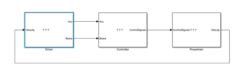
In this forward model of the conventional vehicle with a 1.9L engine and a 4-speed automatic transmission, there are three main blocks representing the driver, controller, and Powertrain, and the signal generated by the powertrain is fed into the driver block which acts as a feedback signal.
Driver Block:
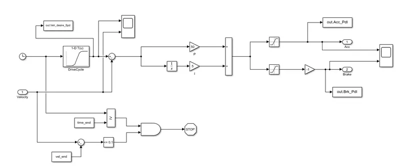
In the driver block, the driver cycle selected from the initialization folder is loaded in this block with the use of the 1D lookup table, and then after subtracting it with the feedback signal for comparison the actual drive cycle with the help of the PI controller is generated and this drive cycle is segregated using the saturation block with limits 0 to +inf for acceleration values and limits 0 to -inf for break pedal values. And also the time comparator is used to stop the simulation after the drive cycle is over.
Controller Block:
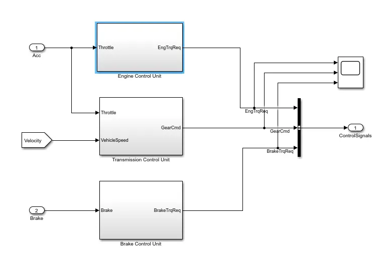
This controller block is divided into three sections Engine Control unit which defines the torque required to be produced by the engine, the transmission control unit which selects the required gear ratio depending upon the feedback velocity signal, and the brake control unit which controls the brake of the vehicle.
Engine Control Unit:
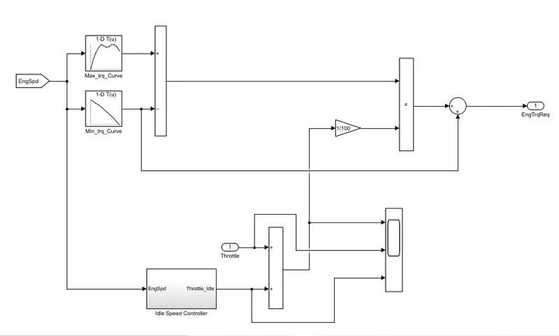
An engine control unit uses the feedback of engine speed from the engine itself i.e. the speed of the engine available after overcoming the inertia and pump load requirements this is fed to two 1D look table which has loaded in it, the max and min torque values from the vehicle data sheet and the values from the 1D lookup table are further subtracted and multiplied with the idle speed value to generate the torque required to be produced by the engine value.
Transmission Control Unit:
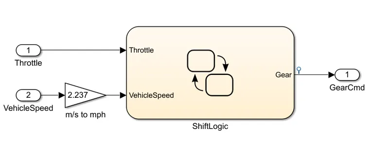
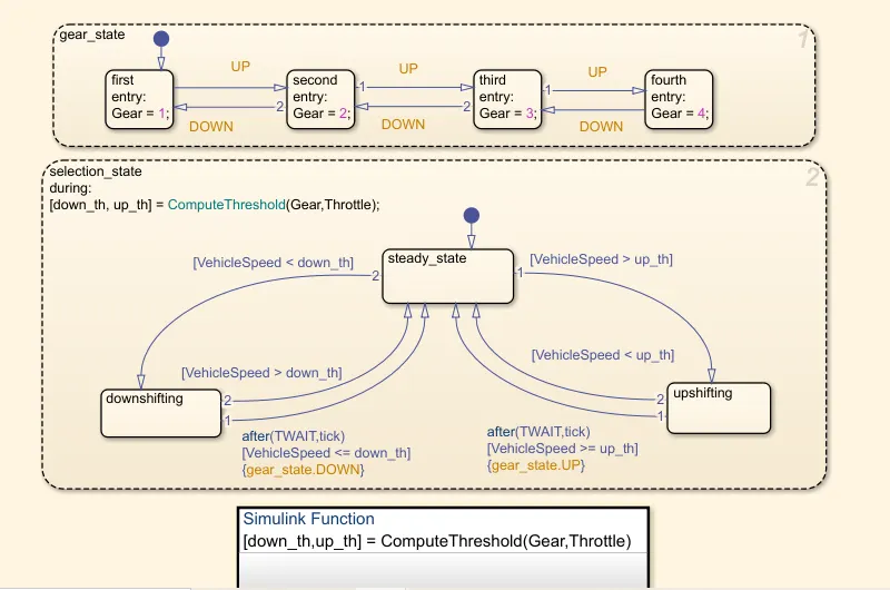
The transmission control unit with help of the shift logic which utilizes the Stateflow to define the logic to shift the gears controls the automatic transmission of the vehicle it uses the acceleration value from the Driver block and Velocity value from the vehicle dynamics section of the Powertrain for applying the logic in the Stateflow.
Brake Control Unit:
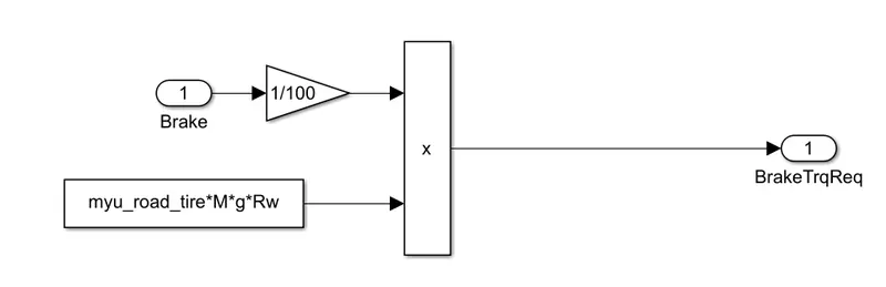
It uses the Brake value from the driver block and rolling resistance of the tire to generate the brake torque required on the wheels.
The commands from the controller are used inside the powertrain of the vehicle to define the actual working of the vehicle. The powertrain consists of five main sections engine, transmission, differential, wheels, and vehicle dynamics.
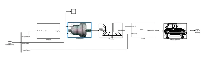
Engine:
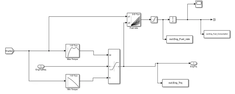
The engine section uses the engine torque required value from the engine controller and the current engine speed value after overcoming inertia and load to look into the Max and Min torque 1D lookup tables which have vehicle torque data loaded in them. And this data from the 1D lookup is then compared with the torque requirement of the engine with the help of a dynamic saturation block the actual torque output of the engine is generated and the fuel consumption rate is an engine is also computed by comparing this output torque data with the vehicle fuel consumption patter loaded inside the 2D lookup table and this rate of fuel consumption is integrated to obtain the total fuel consumption value over time.
Transmission:
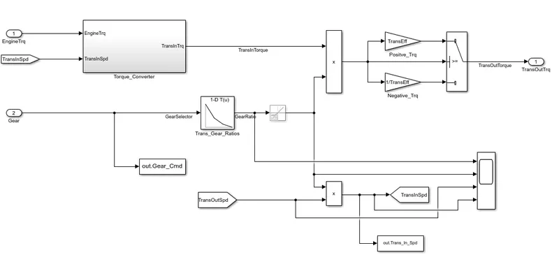
In the transmission block, the torque converter section uses the torque generated by the engine and the transmission input speed of the shaft to generate the required torque using the vehicle data from the 1D lookup tables of the k factor and torque ratio. And the transmission torque is multiplied by the gear ratio and based on the negative torque or positive torque its efficiency is selected to generate the actual transmission torque output.
Differential:
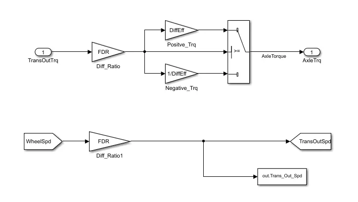
In the differential section, the torque from the transmission is multiplied by the differential ratio, and based on the positive or negative torque its efficiency is multiplied with the use of the switch selector and the axel torque is defined. The transmission output is calculated by multiplying the speed of the wheels with the differential ratio.
Wheels:
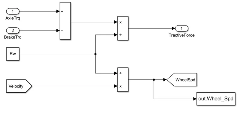
The tractive force available at the wheels is calculated by dividing the rolling radius of the wheels from the value obtained by subtracting the brake torque value from the Axle torque. And the speed of the wheels is calculated by dividing the velocity of the vehicle by the rolling radius of the wheel.
Vehicle Dynamics:
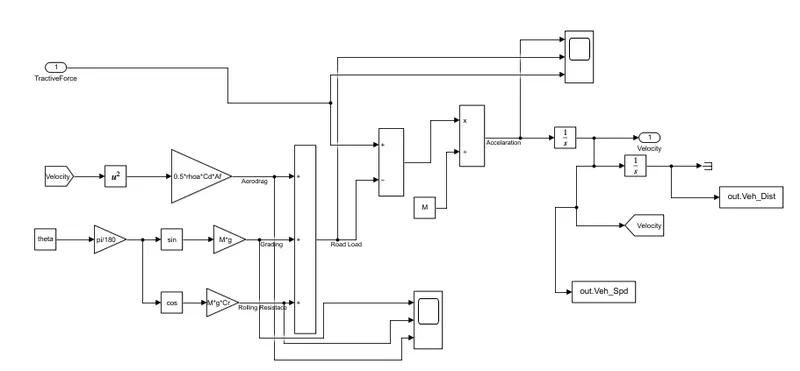
In the vehicles dynamics section, the tractive force at the wheels is subtracted with the road load which is a collective load from the aero drag, grading force, and rolling resistance of the vehicle, and this subtracted value is multiplied by the mass of the vehicle to obtain the acceleration of the vehicle and the acceleration of the vehicle is integrated to obtain the velocity of the vehicle and this velocity of the vehicle is further integrated to obtain the distance traveled by the vehicle over time.
The values from this Simulink model are transferred back to the Matlab script with the use of the To Workspace block and the postprocessing script is used to plot all the results of the vehicle as per the challenge.
%% Renaming variables
Time = out.tout;
Acc_Pdl = out.Acc_Pdl;          % Accelerator pedal [%]
Brk_Pdl = out.Brk_Pdl;          % Brake pedal [%]
Gear_Cmd = out.Gear_Cmd;        % Transmission gear
Trans_In_Spd = out.Trans_In_Spd*30/pi;  % Transmission input speed [rpm]
Trans_Out_Spd = out.Trans_Out_Spd*30/pi;% Transmission output speed [rpm]
Eng_Trq = out.Eng_Trq;          % Engine brake torque [Nm]
Eng_Spd = out.Eng_Spd*30/pi;    % Engine speed [rpm]
Eng_Fuel_Consump = out.Eng_Fuel_Consumption;    % Engine fuel consumption [g]
Veh_Dist = out.Veh_Dist/1000;   % Distance traveled by vehicle [km]
Veh_Spd = out.Veh_Spd*18/5;     % Vehicle speed [kmph]
Eng_Fuel_rate = out.Eng_Fuel_rate;  %Fuel consumption rate[g/s]
Veh_desire_Spd = out.Veh_desire_Spd*18/5;    %Speed of the drive cycle[kmph]
Wheel_Spd = out.Wheel_Spd*30/pi;      %Wheel Speed in [rpm]


%% Data Analysis
Eng_Pwr = (Eng_Spd.*pi/30).*(Eng_Trq./1000);   % Engine brake power [kW]
rho_petrol = 0.7197;                    % Density of petrol [kg/L]
kmpl = Veh_Dist(end)/(Eng_Fuel_Consump(end)/1000/rho_petrol);    % Fuel economy [kmpl]


%% Plotting vehicle characteristics time trace
figure()
subplot(4,1,1)
hold on
grid on
plot(Time, Acc_Pdl, 'linewidth', 1, 'Color', 'black');
plot(Time, Brk_Pdl, 'linewidth', 1, 'Color', 'red');
ylabel('Pedal [%]')
xlim([0, Time(end)]);
legend('Accel','Brake');
title('Acceleration and Brake value')
subplot(4,1,2)
hold on
grid on
plot(Time, Veh_Dist)
ylabel('Distance [km]')
xlim([0, Time(end)]);
title('Distance Travelled')
subplot(4,1,4)
hold on
grid on
plot(Time, Gear_Cmd, 'linewidth', 1, 'Color', 'black');
xlim([0, Time(end)]);
xlabel('Time [s]');
ylabel('Gear');
title('Gear No.')
subplot(4,1,3)
hold on
grid on
plot(Time,Veh_Spd,'Color','r')
plot(Time,Veh_desire_Spd,'Color','k')
xlim([0, Time(end)]);
ylabel('Speed [kmph]')
title('Actual vs Desired Speed')
legend('Actual Speed','Desired Speed')

%% Plotting engine operating points on engine fuel map
figure('Name','Engine Operating Points');
hold on
grid on
title('Engine Operating Points','fontsize',12);
p1=plot(Eng_map_spd*30/pi,Eng_max_trq,'linewidth',2,'color','r');
p2=line([Eng_map_spd(end)*30/pi Eng_map_spd(end)*30/pi],[0 Eng_max_trq(end)]);
set(p2,'linewidth',1,'linestyle','--','color','k');
p3=line([Eng_map_spd(1)*30/pi Eng_map_spd(1)*30/pi],[0 Eng_max_trq(1)]);
set(p3,'linewidth',1,'linestyle','--','color','k');
[c,h] = contour(Eng_map_spd'*30/pi,Eng_map_trq,Eng_fuel_map');
clabel(c,h);
xlabel('Engine Speed [rpm]');
ylabel('Engine Torque [Nm]');
title('Engine Fuel Consumption Map [g/s]');
p4 = plot(Eng_Spd,Eng_Trq,'.','color','k');
legend([p1 p4],{'Max Curve','Operating Points'});
axis([Eng_map_spd(1)*30/pi Eng_map_spd(end)*30/pi 0 Eng_map_trq(end)]);

figure()
subplot(4,1,3)
hold on
grid on
plot(Time,Eng_Fuel_rate)
xlim([0, Time(end)]);
ylabel('Fuel Rate[gm/s]')
title('Fuel rate')
subplot(4,1,4)
plot(Time,Eng_Fuel_Consump)
hold on
grid on
xlim([0, Time(end)]);
ylabel('Fuel [g]')
xlabel('Time [s]')
title('Fuel Consumption in gm')
subplot(4,1,1)
hold on
grid on
plot(Time,Eng_Trq)
xlim([0, Time(end)]);
ylabel('Torque [Nm]')
title('Engine torque in Nm')
subplot(4,1,2)
hold on
grid on
plot(Time,Eng_Pwr)
xlim([0, Time(end)]);
ylabel('Power [kw]')
title('Engine Power in kw')

figure()
plot(Time,Trans_Out_Spd,'Color','r')
hold on
grid on
plot(Time,Trans_In_Spd,'Color','k')
plot(Time,Wheel_Spd,'Color','b')
xlim([0, Time(end)]);
ylabel('Speed [rpm]')
xlabel('Time [s]')
legend('Trans Out', 'Trans In', 'Wheel Speed')
Comparison of UDDS and HWFET cycle:
UDDS Plot
HWFET Plot
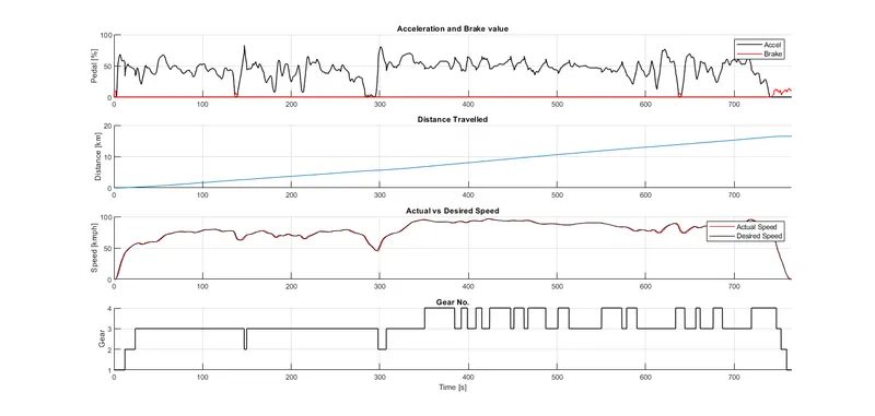
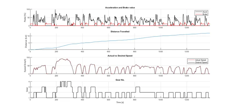
Here it can be clearly seen that the urban drive runs at lower speed and requires lower gears with higher torque ratios to fulfill its high acceleration demand compared to the highway drive cycle which has less braking conditions and runs on higher gear numbers with low torque ratios. And the vehicle in the highway drive cycle covers more distance i.e. about 16km in 800secs while the distance traveled by the vehicle in the urban drive is about 14km in 1300secs and both the vehicle uses the same quantity of the fuel i.e. 700gms of fuel which can be seen the plot no. 4 below hence the HWFET drive cycle is much more efficient compared to the UDDS cycle.
Fuel Consumption Map of UDDS cycle
Fuel Consumption Map of HWFET cycle
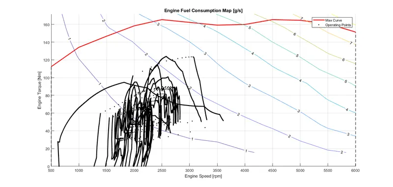
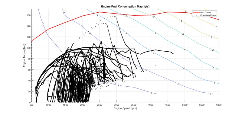
Here from the operating points of the engine, it can be seen that the HWFET cycle consumes less fuel and performs more efficiently by operating at lower engine speeds and lower engine torque compared to the urban drive cycle which operates the engine at higher speeds and higher torque hence being less efficient and consuming more fuel.
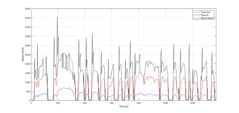
Speeds plot of the UDDS cycle
Speeds plot of HWFET cycle
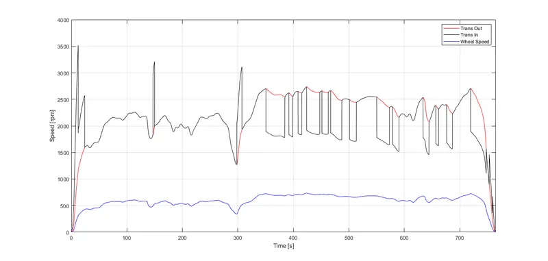
It can be seen that the transmission output speed of the highway drive cycle is higher than its transmission input speed hence less effort is required to move the vehicle forward which results in faster wheel speed, while in the urban drive cycle the transmission output speed is lower than the transmission output speed so more effort is required to move the vehicle forward and so the wheels move at a lesser speed.
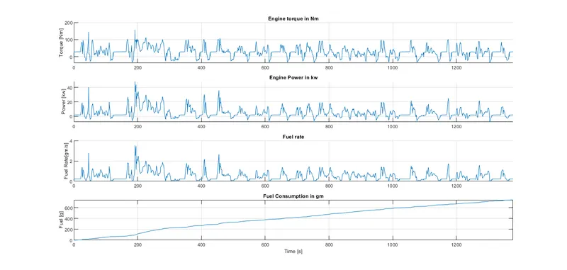
UDDS Cycle plot
HWFET cycle plot
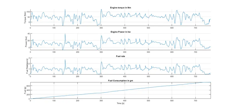
In the above plot, it can be seen that the operating power and torque of the engine in the highway drive cycle are less compared to the urban drive cycle and the fuel consumption of both cycles is almost equal at 700gms but the distance traveled by the vehicle in the highway is about 16km and that in the urban drive cycle is about 14km in higher time span this indicates that the efficiency of the highway drive cycle is far better than the urban drive cycle as it has less break torque being applied on the wheels which reduces the overall torque requirement on the engine and provide it better operating conditions to perform efficiently.