Project 1

2. b)

Mini-Batch Gradient Descent:

Algorithm-

Let theta = model parameters and max_iters = number of epochs.

for itr = 1, 2, 3, …, max_iters:
for mini_batch (X_mini, y_mini):

• Forward Pass on the batch X_mini:
  • Make predictions on the mini-batch
  • Compute error in predictions (J(theta)) with the current values of the parameters
• Backward Pass
• • Compute gradient(theta) = partial derivative of J(theta) w.r.t. theta
• Update parameters:
  • theta = theta – learning_rate*gradient(theta)

the Python Implementation:

Step #1: First step is to import dependencies, generate data for linear regression and visualize the generated data. We have generated 8000 data examples, each having 2 attributes/features. These data examples are further divided into training set (X_train, y_train) and testing set (X_test, y_test) having 7200 and 800 examples respectively.

# importing dependencies
import numpy as np
import matplotlib.pyplot as plt
  
# creating data
mean = np.array([5.0, 6.0])
cov = np.array([[1.0, 0.95], [0.95, 1.2]])
data = np.random.multivariate_normal(mean, cov, 8000)
  
# visualising data
plt.scatter(data[:500, 0], data[:500, 1], marker = '.')
plt.show()
  
# train-test-split
data = np.hstack((np.ones((data.shape[0], 1)), data))
  
split_factor = 0.90
split = int(split_factor * data.shape[0])
X_train = data[:split, :-1]
y_train = data[:split, -1].reshape((-1, 1))
X_test = data[split:, :-1]
y_test = data[split:, -1].reshape((-1, 1))
  
print("Number of examples in training set = % d"%(X_train.shape[0]))
print("Number of examples in testing set = % d"%(X_test.shape[0]))

Output: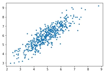

3. C)

Stochastic Gradient Descent (SGD):

The word ‘stochastic‘ means a system or a process that is linked with a random probability. Hence, in Stochastic Gradient Descent, a few samples are selected randomly instead of the whole data set for each iteration. In Gradient Descent, there is a term called “batch” which denotes the total number of samples from a dataset that is used for calculating the gradient for each iteration. In typical Gradient Descent optimization, like Batch Gradient Descent, the batch is taken to be the whole dataset. Although, using the whole dataset is really useful for getting to the minima in a less noisy and less random manner, but the problem arises when our datasets get big.

SGD algorithm:

So, in SGD, we find out the gradient of the cost function of a single example at each iteration instead of the sum of the gradient of the cost function of all the examples.

In SGD, since only one sample from the dataset is chosen at random for each iteration, the path taken by the algorithm to reach the minima is usually noisier than your typical Gradient Descent algorithm. But that doesn’t matter all that much because the path taken by the algorithm does not matter, as long as we reach the minima and with a significantly shorter training time.

def SGD(f, theta0, alpha, num_iters):
    """
       Arguments:
       f -- the function to optimize, it takes a single argument
            and yield two outputs, a cost and the gradient
            with respect to the arguments
       theta0 -- the initial point to start SGD from
       num_iters -- total iterations to run SGD for
       Return:
       theta -- the parameter value after SGD finishes
    """
    start_iter = 0
    theta = theta0
    for iter in xrange(start_iter + 1, num_iters + 1):
        _, grad = f(theta)
  
        # there is NO dot product ! return theta
        theta = theta - (alpha * grad)

1. A)

Batch Gradient Descent: Batch Gradient Descent involves calculations over the full training set at each step as a result of which it is very slow on very large training data. Thus, it becomes very computationally expensive to do Batch GD. However, this is great for convex or relatively smooth error manifolds. Also, Batch GD scales well with the number of features.

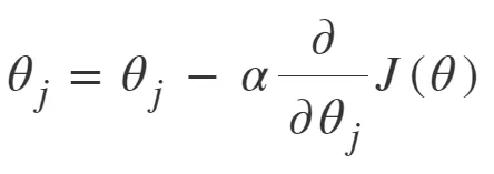
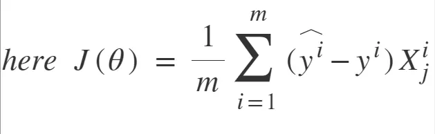
Algorithm for batch gradient descent :
Let h_θ(x) be the hypothesis for linear regression. Then, the cost function is given by:
Let Σ represents the sum of all training examples from i=1 to m.

Jtrain(θ) = (1/2m) Σ( hθ(x(i))  - y(i))2

Repeat {
 θj = θj – (learning rate/m) * Σ( hθ(x(i))  - y(i))xj(i)
    For every j =0 …n 
}
Where xj(i) Represents the jth feature of the ith training example. So if m is very large(e.g. 5 million training samples), then it takes hours or even days to converge to the global minimum.That’s why for large datasets, it is not recommended to use batch gradient descent as it slows down the learning.