A)Importing the necessary libraries and the raw data

import pandas as pd
import numpy as np
import matplotlib.pyplot as plt

df = pd.read_csv('auto.csv')
df.head()

print(df.dtypes)


B)Basic insight from data

print(df.dtypes)


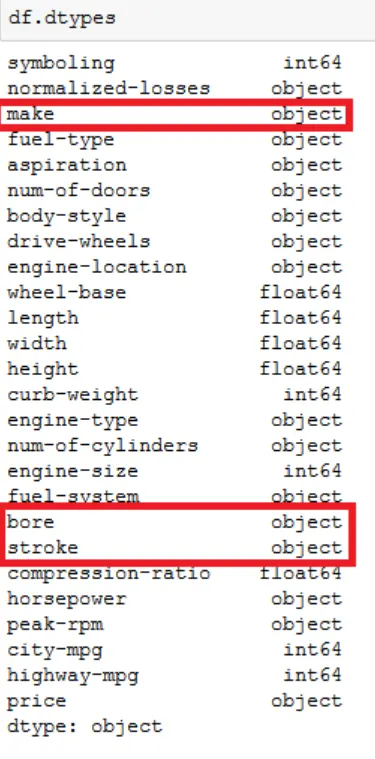
In the above picture, the make is the brand name of the car it is supposed to be an object.
But bore and stroke which are supposed to be in number. To change it from object to number, data formatting take place.

• Data Distribution

we have to check the statistical summary of each column to learn about the distribution of data in each column. The statistical measures can tell that there are any mathematical issues that may exist, such as extreme outliers and large deviations.

To get the quick statistics, we use the describe method df.describe() .

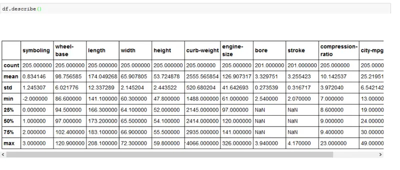
It returns the number of terms in the column as “count”, average column value as “mean”, column standard deviation as “std”, the maximum and minimum values, as well as the boundary of each of the quartiles.
By default, the dataframe.describe() function skips rows and columns that do not contain numbers.

The describe() method return summary for numbers, to get a summary of all the column with the object data-type we could add an argument “ include = “all” “ inside the describe function bracket.

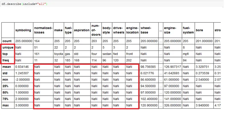
Unique” is the number of distinct objects in the column, “top” is the most frequently occurring object, and “freq” is the number of times the top object appears in the column. Some values in the table are shown here as “NaN”, which stands for “not a number”. This is because that particular statistical metric cannot be calculated for that specific column data type.

Data cleaning:

Data cleaning is a data per-processing process which is a necessary step in data analysis.

• Dealing with missing values

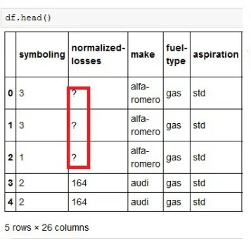
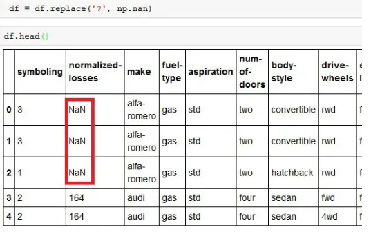
When no data value is stored for a feature for a particular observation, we say this feature has a “missing value”. Usually, missing value in data-set appears as “?”, “NaN”, 0 or just a blank cell.

• Drop missing values

To remove data that contains missing values, pandas library has a built-in method called “dropna”. Essentially, with the dropna method, you can choose to drop rows or columns that contain missing values, like NaN. We have to specify “axis=0” to drop the rows, or “axis=1” to drop the columns that contain the missing values.

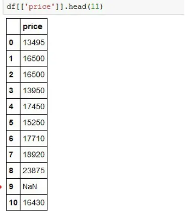
There are some missing values in “Price”. Since the price of used cars is what we’re trying to predict in our upcoming analysis. we have to remove the cars(the rows) that don’t have a listed price.

To do so we have to use: df.dropna(subset=[“price”], axis=0,inplace=True)

• Drop missing values

To remove data that contains missing values, pandas library has a built-in method called “dropna”. Essentially, with the dropna method, you can choose to drop rows or columns that contain missing values, like NaN. We have to specify “axis=0” to drop the rows, or “axis=1” to drop the columns that contain the missing values.

There are some missing values in “Price”. Since the price of used cars is what we’re trying to predict in our upcoming analysis. we have to remove the cars(the rows) that don’t have a listed price.

To do so we have to use: df.dropna(subset=[“price”], axis=0,inplace=True)

Drop missing (“NaN”) values from Price column

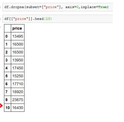
The arguments “subset=[[‘Specific_column_name’]]”, “axis=0” to drop the rows, or “axis=1” to drop the columns, “inplace= True” allows the modification to be done on the data-set directly.

• Replace missing values : Replacing data is better, since no data is wasted.

Data we were dealing with have both numerical and categorical data.
I)In numerical data missing values can be replaced with the “average” of the values that the columns have.
II) While in categorical data missing value can be handled with “Mode” (frequently occurring) value.

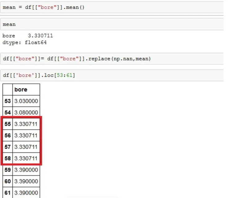
To replace missing values like “NaN” with actual values, pandas library has a built in method called ‘replace’, which can be used to fill in the missing values with the newly calculated values.

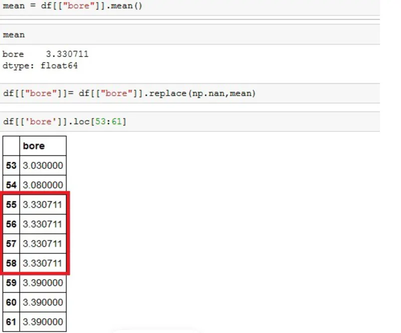
To replace the missing values of the column‘Bore’ by the mean value of the variable. Therefore, the missing value should be replaced by the average of the entries within that Column.

• Data Formatting

Data formatting means bringing data into a common standard of expression that allows users to make meaningful comparisons.

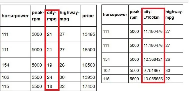
In our used car data-set, there’s a feature named “city-mpg” in the data-set, which refers to a car fuel consumption in miles per gallon unit. However, we don’t use such mpg, we want to convert those values to L/100km — the metric version. L / 100km = 235.21/ x mpg

df[['city-mpg']]=235/df[['city-mpg']]
df.rename(columns={'city-mpg':'city-L/100km'},inplace=True)

In the second line of code, rename column name from “city-mpg” to “city-L/100km” using the dataframe.rename() method

Dealing with incorrect datatype :Sometimes the wrong datatype is assigned to a feature.

df[['price']].dtypes

Out: price object

dtype: object

Here data type to the price feature is “object” the expected data type should really be an integer or float type.

To covert datatype: dataframe.astype()

Binning :

In the actual car data-set, “price” is a numerical variable ranging from 5,188 to 45,400, it has 201 unique values. We can categorize them into 3 bins: low, medium, and high-priced cars.

binwidth = int(max(df['price']) min(df['price']))/3)
bins = range(int(min(df['price'])),int(max(df['price'])),binwidth)
df['price-binned']=pd.cut(df['price'],bins,labels=["low","medium","High"])
df.loc[15:20,['price','price-binned]]
df['price-binned'].dtypes

• Turning categorical variables into quantitative variables

Most statistical models cannot take in objects or strings as input, it only take the numbers as inputs.

In the car data-set, the “fuel-type” feature as a categorical variable has two values, “gas” or “diesel”, which are in String format. For further analysis, it has to convert into some form of numeric format. In the case where the feature “Fuel” has two unique values, gas and diesel, we create two new features ‘gas’ and ‘diesel.’

dummy_variable = pd.get_dummies(df['fuel-type])

dummy_variable.rename(columns={'fuel-type':'gas','fuel-type:diesel'},inplace=True)

df=pd.concat([df,dummy_variable],axis=1)

df.drop("fuel-type",axis=1,inplace=True)

df.head()

Boxplots:

Boxplots are a great way to visualize numeric data, since you can visualize the various distributions of the data.

The main features that the boxplot shows the “median” of the data, which represents where the middle datapoint is. The Upper Quartile shows where the ”75th percentile” is, the Lower Quartile shows where the “25th percentile” is. The data between the Upper and Lower Quartile represents the Interquartile Range(IQR). Next, you have the Lower and Upper Extremes. These are calculated as 1.5 times the interquartile range above the 75th percentile, and as 1.5 times the IQR below the 25th percentile.
Finally, boxplots also display “outliers” as individual dots that occur outside the upper and lower extremes. With boxplots, you can easily spot outliers
and also see the distribution and skewness of the data.

import seaborn as sns
sns.boxplot(x="drive-wheels",y="price",data=df)
plt.show()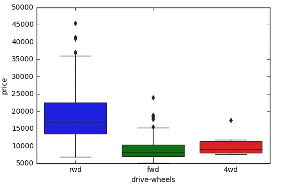

Scatter plot:

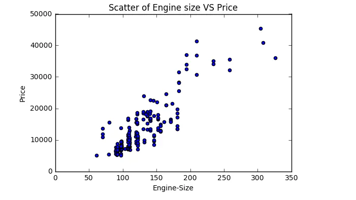
This plot shows the relationship between two variables:

• The predictor variable: is the variable that you are using to predict an outcome. In this case, our predictor variable is the engine size.
• The target variable: is the variable that you are trying to predict. In this case, our target variable is the price, since this would be the outcome.

x=df['engine-size']
y=df['price']
plt.scatter(x,y)
plt.title("scatter of Engine Size VS price")
plt.xlabel('Engine-Size')
plt.ylabel('Price')
plt.show()