Project 1
Title:
Deals with the development of a forward energy-based fuel consumption model of a conventional vehicle.
Aim:-
1) Build Simulink model using blocks and complete the vehicle model
2) wrtting scripts in MATLAB to load all the variables required for running the simulink model
3) Tabulate the fuel economy numbers (kmp) for UDDS and HAFET cycle
4) Polt the time trace for engine transmission input transmission output and wheel speed on one plut
5) Plot engine torque, engine power fuel rate and fuel consumption using subplots
6) Plot accelerator and brake pedal, gear command vehicle desired and actual speed, vehicle distance using subplots
7) Plot the engine operating points on the engine fuel map
8) Generate the plots for both drive cycles
9) Study of Conventional vehicle simulink model and creates graphs
Conventional Vehicle:-
Conventional vehicles use an internal combustion engine fueled by gasoline or diesel to power the wheets in this the heat engine uses the principle of heat release through combustion of a fuel with an oxidizer in a combustion chamber to create expanding gases which pushes against a piston creating force and torque output
In this vehicle engine converts chemical energy stored in the fuel into heat which is used to produce useful work Typically use fossil fuels like petroleum (potrol and diesel)
The most popular type of engine is used in this system is 4 stroke reciprocating engine Engine in cyclinder process can be represented by ideal thermodynamic cycles such as Otto cycle Diesel cycle. Otto cycle is a ideal cycle thet describes the cyce process for spark ignited SI engine and the Diesel cycle is the ideal cycle thet describes the cycle process for a compression ignited CI engine
Energy and performance of vehicle:-
In this system trge power demand on the wheel need to instant supplied by the powertrain. In otyher word the power coming from the powertrain dictates the power demand on the wheels (as per performance viz, acceleration, speed etc is determined by it.
In tis vehicle the powertrain is consists of an engine connected to the wheels through a transmission therefore the power comes from the engine through the transmission.
Conventional powertrain efficiency:-
The engine generates power by converting chemical energy stored into the mechanical energy by the process of combustion. This process of energy conversion also has an efficiency and the energy input is in the form of fuel consumption.
- Instantaneous fuel consumption is given as
where,
mf = mass flow rate in [kg]
pe = power of engine
pt = power of transmission
nt = efficiency of transmission
ne = efficiency of engine
QLHV = it is the ecalorific value / lower heating value of fuel
In this system of IC engine if tge power at the wheels is zero the engine is idling and still consumes some fuel to overcome the engine drag loss and keep it spinning this is the idling fuel consumption and know as idling process. Above mentioned formula is applicable only when the wheel power is strictly power. When the wheel power is negative either th engine is disengaged and idling or the engiune is engaged and providing some engine braking due to the engine. drag losses.
The engine is consuming fuel when it is idling but even for engine braking the engine might be consuming some fuel.
The fuel consumption not only depend on the power requirement at the wheels but also is - required to generate power to run the various engine and vehicle accessory loads.
System Dynamics:-
It deals with the modeling of multi domain systems through the use of a unified approach based on a ordinary differential and algebraic equation describing the static and dynamic
effects. Each systems has are two generalised variables
1) Efforts:- It is generalised force variable. ex torque, force, voltage, heating value.
2) Flow:- It is the generalised flow/velocity variable, ex-velocity, current mass flow rate.
3) power:- it is the product of the effort and flow variable it is interchangeable between energy domains
Energy based models- Element models
To models the internal physical properties of the element and the losses there are basically two kinds of approach
1] Map based models:- Elements are modeled using maps which characterized the relationship between the input and output, output and losses etc.
2] Analytical models:- Elements are modeled using physical equation that represent the internal dynamics. These are the two extremes most models are a combination of the two with some dynamics models analytically and for some using maps.
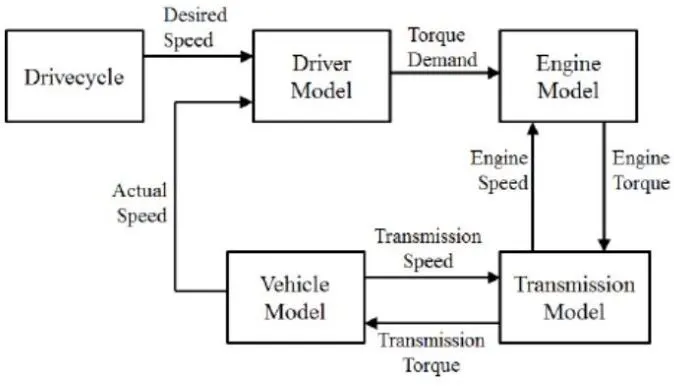
In this model We use Forward Model
It also known as dynamic simulation. Dynamic models are used for detailed simulations. In this model force/torque/power is the input and the vehicle state variable velocity and acceleration. are outputs. The models and simulatios are more realistic due to phhysical casualty hence. appropriate for control development. There is feedback loop to meet the desired vehicle state. It is mainly used to simulate a vehicle on a driving cycle to analyse the dynamic behaviour of the system helps significantly in control development.
MATLAB scripts:-
Used to load all the variables required for running the Simulink model and for post-processing. The drive cycle selection is also done here. Before running the Simulink vehicle model, run this initialization script.
%%%%%%%%%%%%%%%%%%%%%%%%%%%%%%%%%%%%%%%%%%%%%%%%%%%%%%%%%%%
%Skill-Lync >> Hybrid Drives Development
%Project 1 - Conventional Vehicle Model
%By - suriyanithi M
%Description:
%%Initialization File
%Initialization file for loading the variables for the Conventional vehicle simulation model
%%Vehicle Parameters
M = 1500; % Vehicle weight [kg]
Cr= 0.015; %Rolling resistance coef
ficient
Rw = 0.35; %rolling radius [m]
Cd = 0.33; %Drag coefficient
Af = 2; %Frontal area [m2]
rhoa = 1.225; % Air density [kg/m3]
Vwind = 0; %Wind velocity [kmph]
9 = 9.81; %Gravitational accelerat.
ion [m/s2]
theta = 0; %Slope [deg]
myu_road_tire = 1; %Coefficient of friction between tire - road interface
%%Powertrain Parameters
FDR = 3.73; %Fin
al Drive Ratio / Diff Ratio
DiffEff = 0.99; %Dif
ferential efficiency (assumed independent of operating conditions)
NumGear = 4; %Num
ber of gears in transmission
TransGear 11 NumGear]; %Tra
nsmission Gears
TransRatio 13.06, 1.62, 1, 0.7]: % Cor
responding Transmission ratios
TransEff 0.90; %Tra
nsmission efficiency (assumed independent of operating conditions)
TC_SR= [0, .5, .6, .7, .8, .87, .92, .94, .96, .97, .1: Torque Converter Speed Ratio (Matlab default) -> Turb5pd/Pumps pd
TC_TR = [2.232, .1.5462, .1.4058, .1.2746, .1.1528, .1.0732, .1.0192, 1, 1, 1, 1]; torque Converter Torque Ratio (Matlab default) TurbTra/PumpTra
TC_Cf = 1e-4 * [.72558, .66322, .63463, .59042, .51331, .4144, .29287, .22444, .12186, .04386, 0]; % Torque Converter Capacity Factor (Matlab default) -> PumpTra/Pu mpSpd 2 [Nm/rpm^2]
Load Vehicle_Data/Engine_data_1_9L_Saturn_95KM
load Vehicle_Data/Trans_Shift_map
%%Driver Parameters
Kp = 10; %P gain for
driver PI model
Ki = 10; %I gain for
driver PI model
Drive_Cycle_Select = 1; %Drive cycle selection
%Drive cycle values in m/s
if Drive_Cycle_Select == 1
load DriveCycles/UDDS;
elseif Drive_Cycle_Select == 2
load DriveCycles/HWFET;
elseif Drive_Cycle_Select== 3
load DriveCycles/FTP;
elseif Drive_Cycle_Select == 4
load DriveCycles/US06;
elseif Drive_Cycle_Select == 5
load DriveCycles/NEDC;
elseif Drive_Cycle_Select == 6
load DriveCycles/WLTP:
end
time_end = cyc_time(end);
vel_end = cyc_vel(end):
NOW,
lets see the simulink model of conventional vehicle :-
in this project, a typical midsize car with a 1.9L engine and a 4-speed automatic transmission is considered Data is taken from ADVISOR data base developed by NREL, USA. Transmission shift map and controller is taken from Matlab/Simulink example database.
The model developed has the capability to simulate the vehicle on different drive cycles like UDDS, HWFET, FTP, NEDC, etc.
"Projectl_InitFile.m" is a Matlab script used to load all the variables required for running the Simulink model and for post-processing. The drive cycle selection is also done here. Before running the Simulink vehicle model, run this initialization script.
Driver Model:-
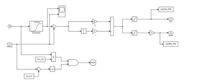
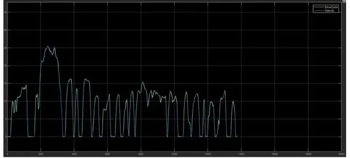
it is modeled using a 'Driver block, which is a basic Pl controller that generates accelerator and brake pedal outputs to match the desired and actual vehicle speeds. In this we use drive cycles fro the based on these results of fuel consumption and emissions the vehicle gets certified and it also forms a basis of uniform asessment. It is based on time, velocity then its all integrate and creates output accelration pedal and brake pedal
Graph created from Scope in Driver Model
Control Model:-
The 'Controller block is the brains of the vehicle, representing the electronic controls units. It is based on the driver inputs, it generates desired engine torque, desired transmission gear and desired brake torque. These inputs are ted to the Powertrain block which represents the drivetrain of the vehicle.
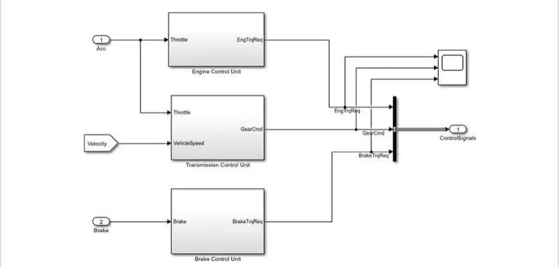
1) engine control unit :-
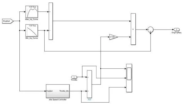
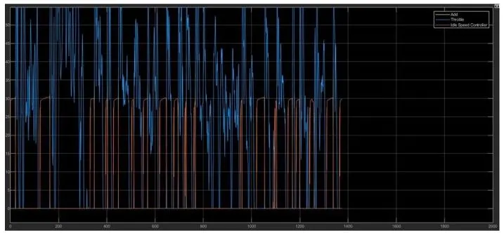
In this control model We use engine control unit in that give input Engine speed through creating look up table, in that table we give input Maximum torque and map speed then also create 2nd look up trable in that give input ct torque and map speed then it substracts and multiplied. the engine speed also give to ideal contro speed to integrate from this we meet output of engine required torque.
Graph created from Scope in Driver Model:
2) Transmission Control Unit:-
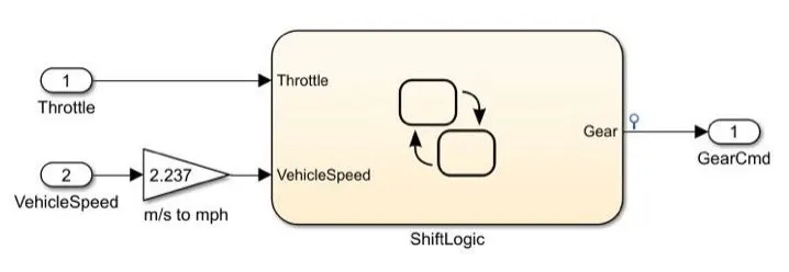
In this unit we create steadfy flow variable state for controlling of gears of vehicle as in ascending and descending order with respect to time, speed, distance, and give input to this steady state is vehicle speed in m/s to mph.
3) Brake Control Unit :-
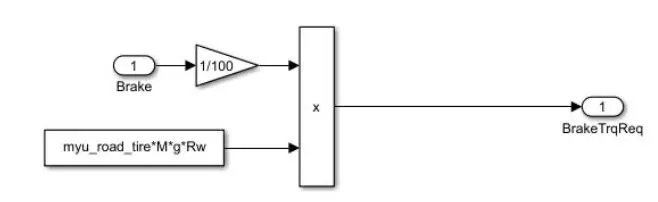
in this calculation brake torque and then all three control signals output is give to powertrain
3) powertrain :-
The powertrain encompasses every component that converts the engine's power into movement. This includes the engine, transmission, the driveshaft, differentials, axles, basically anything from the engine through to the rotating wheels.
1 Engine:-
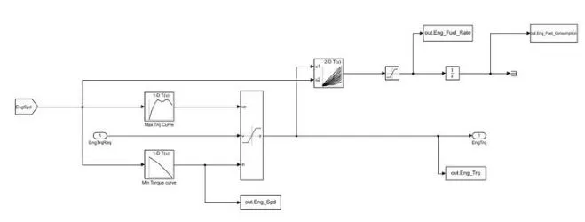
In this model we used map based model to model the fuel consumption of engine. It is based on maximum Torque and minimum torque from the controller. and then it saturated torque and give output then saturated torque and speed map give fuel consumption takes the speed and torque then the output goes into saturated then its integrated.
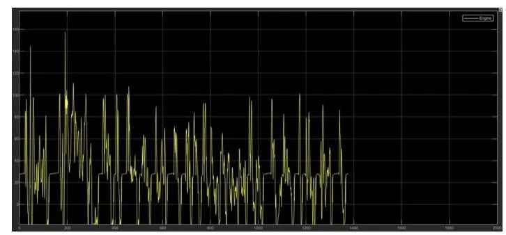
Graph created from Scope in Driver Model Engine Torque :-
engine torque
2)transmission :-
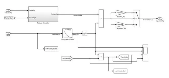
In these model we take engine torque, gear selector from controllerb for transmission of gear ratio. The ratio is multiply by transmission input torque and then the transmission efficiency positive torque and negative torque gives transmission input speed. In this case torque converter connects the engine to transmission it is part of transmission. In it basically engine dynamics and that is decoupled.
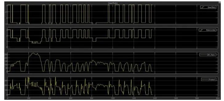
Graph created from Scope in Driver Model:-
1] Transmission in speed 2] Gear ratio 3] Differential
Ratio
3] Differential:
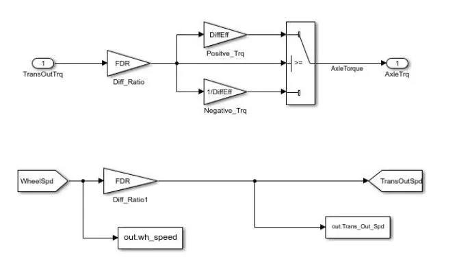
in this taking input is the transmission output then its going to the differential ratio multiplied the output and input torque then meet axle torque. The axle torque is a lower than the transmission torque and differential ratio.
4) Wheels :-
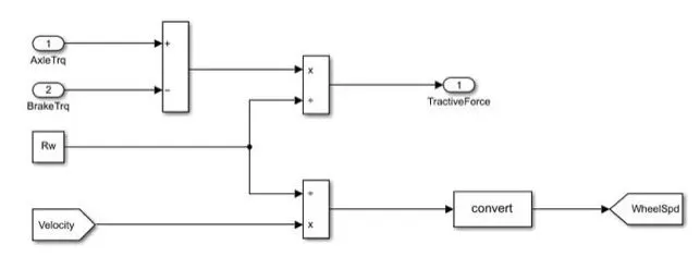
In this model we take the axle torque from differentail and brake torque from controller, it is substracts and multiplied rolling radius and velocity then we meet the tractive force from axle and brake torque and the wheelspeed is meet using velocity.
5) Vehicle Dynamics :-
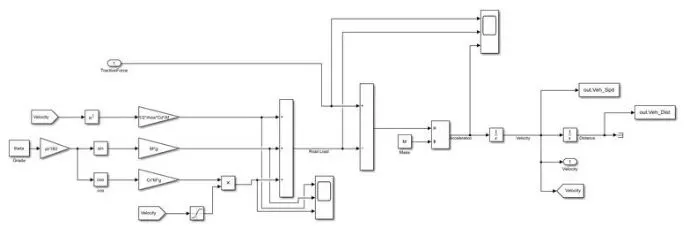
In this takes tractive force and road load It is dictates vehicle speed based on tractive force and road load
the dynamic equation for calculating road food is
where,
P = air density [kg/m^3]
A = frontal area [m^2]
cd = drag coefficient
Vveh = velocity of vehicle [m/s^2]
Vwind = velocity of wind [m/s^2]
cr = rolling resistance coefficient
M = mass in[kg]
g = gravity
then we calculate and integrate then we meet acceleration of vehicle and velocity of vehicle it mean vehicle distance and vehicle speed
graph creating from scope in drive mode :-
1) road load 2) acceleration 3) tractive force
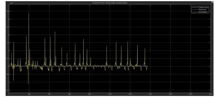
graph creating from scope in drive mode :-
1) road load
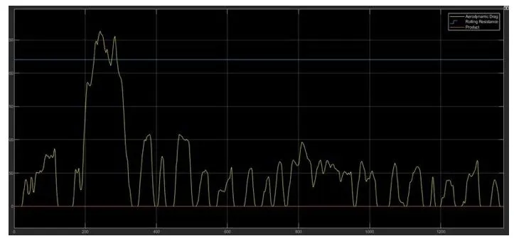
now
we compute the fuel economy numbers using UDDS and HWFET cycle :-
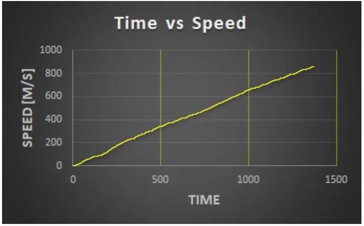
1.) UDDS drive cycle
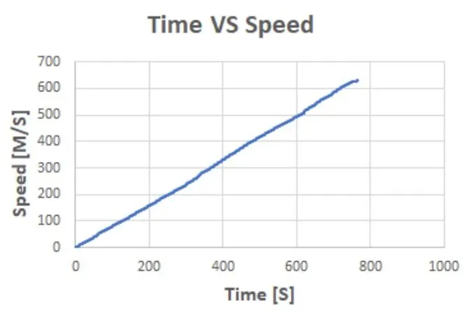
1) time vs speed :- in this the speed is increasing continuously
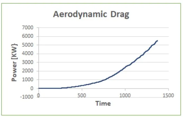
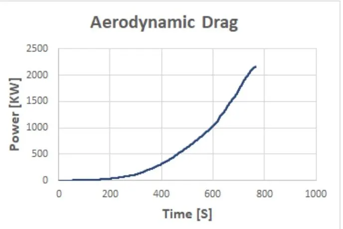
2) aerodyanamic drag :- drag as increase when the power increase
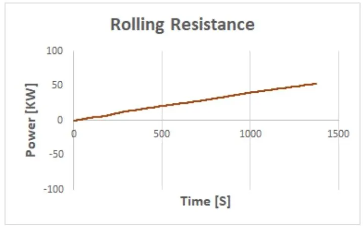
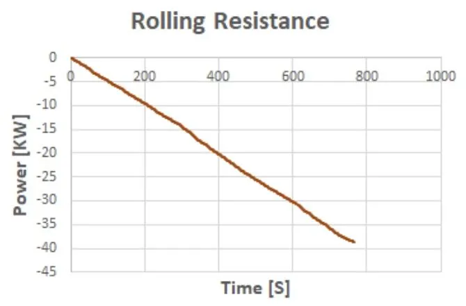
3) rolling resistance :- its also increase when power is increase wrt time
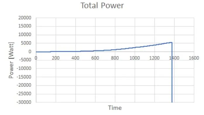
4) total power = aerodynamic drag + rolling resistance + inertial resistance
conclusion :-
total power increase slowly as increasing rolling resistance aerodynamic drag and inertial resistance
2.) HWFET drive cycle :-
1) time vs speed :- speed is continuosly increase wrt time
2) aerodynamic drag :- drag as increase when the power increase
3) rolling resistance :- in this resistance is decrease wrt time
4) total power :- aerodynamic drag + rolling resistance + inertial resistance
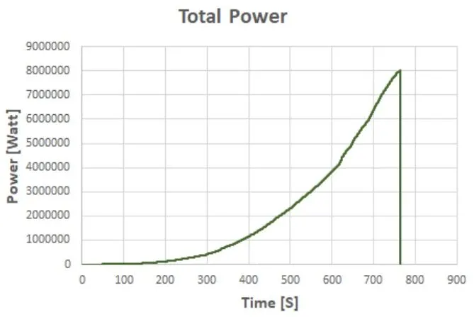
Conclusion:-
Total Power is increase slowly as increasing aerodynamic drag and inertial resistance, but in this drive cycle bad impact occurs due to decreasing rolling resistance.
Result:-
As comparing both cycles we used to UDDS drive cycle. Its best for asses of fuel consumption and Pollutants emission of vehicle in a normalised way
Now For creating Plots we use MATLAB coding So the coding will give down:-
%%%%%%%%%%%%%%%%%%%%%%%%%%%%%%%%%%%%%%%%%%%%%%%%%%%%%%%%%%%
%% SKILL-Lync -> Hybrid Drives Development
%Project 1 - Conventional Vehicle Model
%By - suriyanithi M
%Description:
%The following file is to used with the Initialization file and Simulink
%results for post-processing of the data
%The file is incomplete, has some examples of how the data is imported.
%into a readable format, data analysis and plotting examples.
%Based on the project task, use commands in a similar format as given
%below, to analyse the data and generate required plots.
%You can change variable names if desire
%Post-Processing File
%File for post-processing the Conventional vehicle simulation model data
%%Renaming variables
Time = out . tout;
Acc_Pdt = out.Acc Pdl; %Acceler
ator pedal (%)
Brk_Pdl = out.Brk Pdl; %Brake p
edal (%)
Gear_Cmd = out.Gear_Cmd; %Transmi ssion gear
Trans_In_Spd = out.Trans_in_spd*30/pi; %Transmission input speed (rpm)
Trans_Out_Spd = out.Trans_out_Spd 30/pi; %Transmission input speed (rpm)
Eng_Trq = out . Eng_Trq; % Engine
brake torque [Nm]
Eng_Spd = out . Eng_Spd*30/pi; %Engine
speed [rpm]
Eng_Fuel_Consump = out.Eng_Fuel_Consumpti on; %Engine fuel consumption [g]
Veh_Dist= out . Veh_Dist/1000; % Distance traveled by vehicle [km]
Veh_Spd = out . Veh_Spd*18/5; %Vehicle speed [kmph]
Wheel_Speed = out . wh_speed; %Wheel speed [kmph]
Eng_Fuel_Rate = out . Eng_Fuel_Rate %Engine fuel rate [%]
%% Data Analysis
Eng_Pwr = Eng_Spd*pi/30*Eng_Trg/1000; %Engine brake power [kW]
rho_petrol = 0.7197; %Density of petrol [kg/L]
kmpl = Veh_Dist(end)/(Eng_Fuel Consump(end)/1000/rho_petrol); % Fuel economy [kmpl]
%%Plotting vehicle characteristics time trace transmission IN/OUT and Wheel Speed
figure (1)
hold on
grid on
plot(Time, Trans_In_Spd, 'linewidth', 1,'Color', 'black');
plot(Time, Trans_Out_Spd, 'linewidth', 1,'Color', 'red');
plot(Time, Wheel_Speed, 'linewidth',1, color', 'blue');
ylable('speed [rpm]')
xlable('time [s]')
xlim([0, time(end)]);
ylim([0, 6000]);
legend ('trans input','trans output'.'wheel speed');
%% Plotting vehicle characteristics time trace to Engine speed, Engine Torque, Engine Power,
% And Engine fuel rate, Engine fuel consumption
% Data conversion from Double Timeseries
Eng_spd = Eng_Spd.Data(:,1); % engine speed
Eng_trq = Eng_Trq.datal(:,1); % engine torque
Eng_pur Eng = Pwr.Data(:,1); % engine power
Eng_fuel_rate = Eng_Fuel_Rate.Data(:,1); % engine fuel rate
Eng_fuel_consumption = Eng_Fuel_Consump.Data(:,1); % engine fuel consumption
Veh_dist = Veh_Dist.Data(:,1): % vehicle distance
Veh_spd = Veh_Spd.Datal(:,1); % vehicle speed
%% Plotting Engine speed, Engine Torque, Engine Power, Engine fuel rate, Engine fuel consumption wrt Time
figure(2)
subplot (2,2,1)
plot (Time, Eng_trq, 'linewidth',1, 'color','black')
xlabel('Time [s]')
ylabel('Torque' [Nm])
legend('Engine Torque')
grid on
subplot (2,2,2)
plot (Time,Eng_pwr, 'linewidth',1,'color','blue')
xlabel('Time [s]')
ylabel('Power [KW]')
legend('Engine Power')
grid on
subplot (2,2,3)
plot (Time, Eng_fuel_rate, 'linewidth',1, "color','red')
xlabel('Time [s]')
ylabel('Fuel Rate [%]')
legend('Engine Fuel Rate')
grid on
subplot (2,2,4)
plot(Time, Eng_fuel_consumption, linewidth,1,'color', 'green')
xlabel('Time [s]')
ylabell('Fuel Consumption')
legend ('Engine Fuel Consumption')
grid on
% Plotting fuel economy Vs Engine Fuel consumption
figure (3)
plot (Eng_fuel_consumption, Eng_fuel_rate,'color', 'r')
xlabel('Fuel consumption')
ylabel('Fuel Rate [%]')
title('Fuel economy Vs Fuel Consumption')
grid on
%% Potting Accelerator pedal, Brake pedal and gear command with respect to time
figure(4)
subplot (2,1,1)
hold on
plot (Time, Acc_Pdl, 'linewidth',1, 'Color', 'black');
plot(Time, Brk_pdl, 'Linewidth', 1, 'Color', 'red');
ylable('pedal [%]');
xlable('time [s]);
grid on
legend('accel','brake');
title('acceleration & brake pedal wrt time')
subplot(2,1,2)
plot(Time, Gear Cmd, 'linewidth', 1, Color', 'black');
xlim(0, Time (end)]);
xlabel('Time [s]');
ylabel('Gear ');
grid on
title('Gear command wrt Time')
%% Plotting gear command vehicle desired with actual speed
figure(5)
subplot (2,1,1)
plot(Veh_spd, Gear_Cmd, 'linewidth' ,1, 'Color', 'black');
xlabel (Speed [rpm]');
ylabel('Gear);
grid on.
title('Gear command wrt vehicle speed')
Subplot (2,1,2)
plot(Veh_dast, Gear_Cmd, 'Linewidth' , 1, Color, 'red');
xlabel('Distance [kmpl]');
ylabel('Gear');
grid on
title('Gear command wrt Distance')
%% Plotting engine operating points on engine fuel map
figure('Name', 'Engine Operating Points');
hold on
grid on
title('Engine Operating Points','font size',12);
p1=plot (Eng_map_spd*30/pi,Eng_max_trq, 'linewidth',2. 'color','r');
p2=line( [Eng_map_spd(end)*30/pi Eng_map_spd(end)*30/pi],[0 Eng_max_trq(end)]); set(p2, 'linewidth',1,'linestyle','--'color', 'k');
p3=line ([Eng_map_spd (1)*30/pi Eng_map_spd (1)*30/pi],[0 Eng_max_trq(1)]);
set(p3, 'linewidth', 1, 'linestyle', '--', 'color', 'k');
[c,h] = contour (Eng_map_spd'*30/pi, Eng_map_trq, Eng_fuel_map');
clabel(c,h);
xlabel('Engine Speed [rpm]');
ylabel('Engine Torque [Nm]');
title('Engine Fuel Consumption Map [g/s]');
legend( [p1 p3], {'Max Curve', 'Operating Points' });
axis( [Eng_map_spd(1)*30/pi Eng_map_spd(end)*30/pi 0 Eng_map_trq(end)]);
1) Plotting vehicle characteristics time trace transmission IN/OUT and Wheel Speed:-
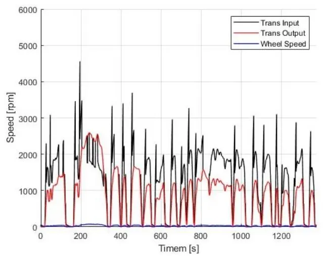
In this graph we see the transmission input and transmission out will fluctuates up and down as increasing speed and time.
2) Plotting vehicle characteristics time trace to Engine speed, Engine Torque, Engine Power, And Engine fuel rate, Engine fuel consumption
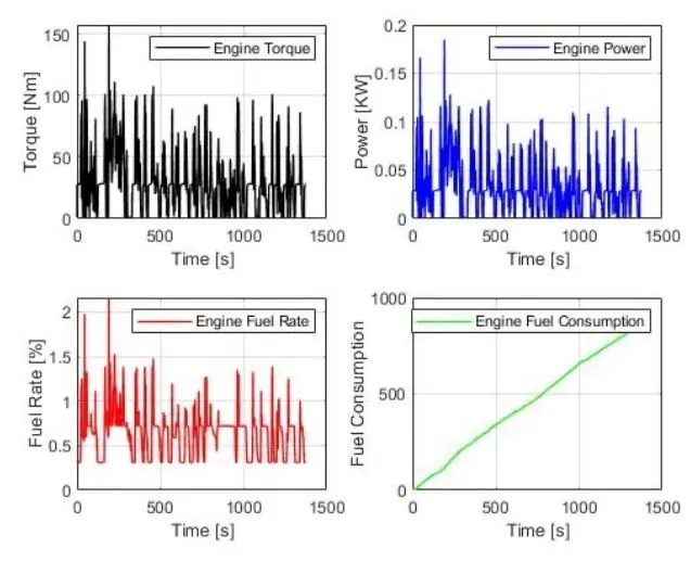
in this engine torque, Engine power, engine fuel rate and engine fuel consumption is increase increasing wrt time.
3) Plotting fuel economy Vs Engine Fuel consumption:-
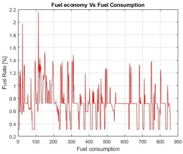
In this the engine fuel consumption is suddenly increase as incresing fuel economy but if fuel economy is constant then the fuel consumption is also constant
4) Potting Accelerator pedal, Brake pedal and gear command with respect to time:-
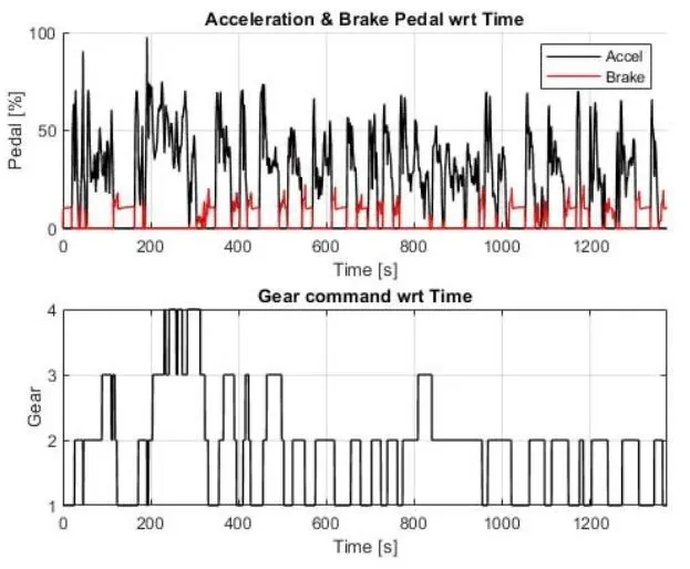
In this the as comparing brake of vehicle the accelaration of vehicle is more so the brake torque is min required, and the gear shifting is also required wrt time
5) Plotting gear command vehicle desired with actual speed:-
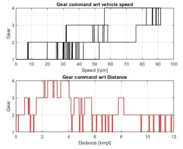
In this the gear shifting is required as increase vehicle speed, as shifting order is gearl, then gear2, then gear3, and then gear4
6) Plotting engine operating points on engine fuel map:-
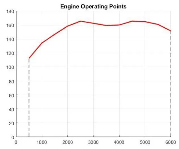
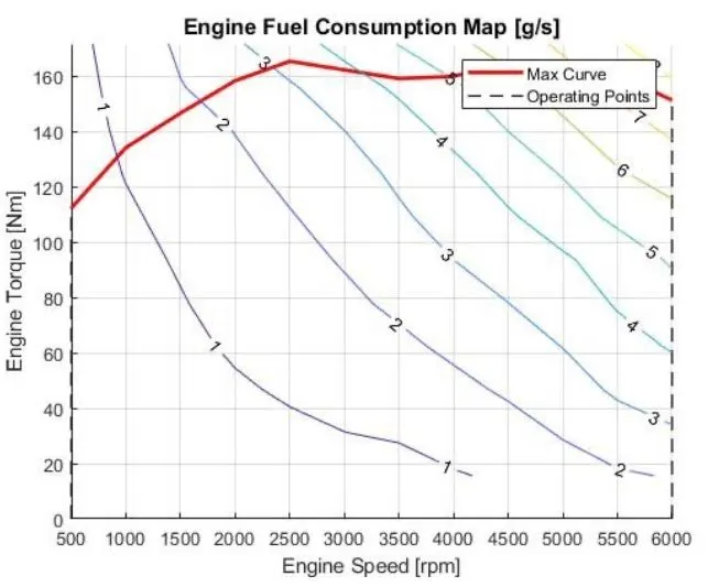
in this the as decrease torque speed is increase
end,,,,,
Thankyou,,,