Project 1
1. Explain the data. Check It is supervised or Unsupervised. Demonstrate?
The data contains the following columns:
<!-- [if !supportLists]-->· <!--[endif]-->age : age of a person
<!-- [if !supportLists]-->· <!--[endif]-->sex : gender of a person
<!-- [if !supportLists]-->· <!--[endif]-->bmi : Body mass index of a person
<!-- [if !supportLists]-->· <!--[endif]-->children : number of children
<!-- [if !supportLists]-->· <!--[endif]-->smoker : if a persons smokes or not
<!-- [if !supportLists]-->· <!--[endif]-->region : region of a person
<!-- [if !supportLists]-->· <!--[endif]-->charges : insurance charges applied
In the supervised learning , If the goal is to predict or estimate the insurance charges based on the given features (age, sex, BMI, children, smoker, and region), then it can be considered a supervised learning problem. In this case, the "charges" column would serve as the target variable or the dependent variable, while the other columns would be the independent variables or features.
In unsupervised learning , In this case we would not have a specific target variable to predict or estimate.
So the above data asumes the goal is supervised learning, but if the objective is different, such as identifying customer segments based on the features, an unsupervised learning approach like clustering algorithms (e.g., k-means, hierarchical clustering) could be used instead.
2. Estimate the minimum sample size n to get the 99�curate predictions. (precision = 0.02)
The minimum sample size n required for 99�curate predictions can be calculated using the formula:
n = (Z^2 * p * (1-p)) / e^2
where Z is the Z-score corresponding to the desired confidence level (for 99% confidence, Z = 2.576), p is the estimated proportion of the population with a particular characteristic (e.g. income, age, etc.), and e is the desired precision or margin of error (e.g. 0.02).
Since the proportion p of the population is unknown, it can be estimated as 0.5. With a precision of 0.02 and Z = 2.576, we get:
n = (2.576^2 * 0.5 * (1-0.5)) / 0.02^2 = 165.67
Therefore, the minimum sample size required for 99�curate predictions with a precision of 0.02 is approximately 166 individuals.
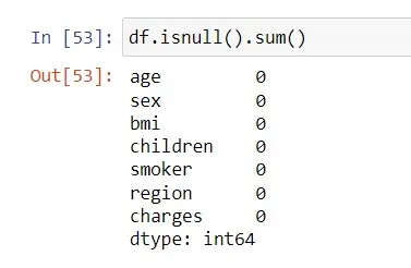
3. Check the data is cleaned or not. If not then clean it (Null values, Row/Column Duplicates, Outliers, Change the string into numbers)
i) check data is cleaned or not
<!--[endif]-->
ii) Check for duplicates
df.duplicated
duplicate_rows = df[df.duplicated()]
num_duplicates = len(duplicate_rows)
# Print the duplicate rows and the count of duplicates
print("Duplicate rows:")
print(duplicate_rows)
print("Number of duplicates:", num_duplicates)

<!--[endif]-->
iii) Convert string to numeric
df.region.replace("southwest", 1, inplace=True)
df.region.replace("southeast", 2, inplace=True)
df.region.replace("northwest", 1, inplace=True)
df.region.replace("northeast", 2, inplace=True)
df.sex.replace("female", 1, inplace=True)
df.sex.replace("male", 2, inplace=True)
df.smoker.replace("yes", 0, inplace=True)
df.smoker.replace("no", 1, inplace=True)
iv) to check outlier
# import matplotlib.pyplot as plt
# plt.boxplot(df)
import matplotlib.pyplot as plt
# Create a box plot
plt.boxplot(df)
# Show the plot
plt.show()
4. Check that sex and smoking are statistically independent or not.
from scipy.stats import chi2_contingency
# Create a contingency table of the two variables
contingency_table = pd.crosstab(df['sex'], df['smoker'])
# Perform the Chi-Square test of independence
chi2, p_value, dof, expected = chi2_contingency(contingency_table)
# Print the test result
print("Chi-Square test statistic:", chi2)
print("p-value:", p_value)
print("Degrees of freedom:", dof)

<!--[endif]-->
Above variables are statistically independent
5. Check that all regressor variables (independent variable) are independent of each other or not.
import seaborn as sns
# Select the regressor variables
regressor_variables = ['age', 'sex', 'bmi', 'children', 'smoker', 'region']
# Create a correlation matrix
correlation_matrix = df[regressor_variables].corr()
# Visualize the correlation matrix as a heatmap
sns.heatmap(correlation_matrix, annot=True, cmap='coolwarm')
# Show the plot
plt.show()
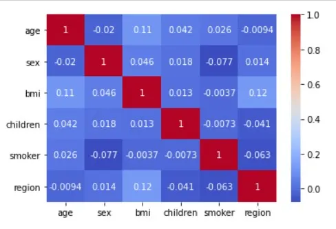
<!--[endif]-->
6. Check the dependency between response and regressors.
<!-- [if !supportLists]-->· <!--[endif]-->To check the dependency between the response and the regressors, you can perform various statistical tests, such as a Pearson correlation coefficient test or a linear regression analysis. The Pearson correlation coefficient test measures the linear relationship between two variables and provides a value between -1 and 1, indicating the strength and direction of the relationship. A value close to 1 indicates a strong positive relationship, a value close to -1 indicates a strong negative relationship and a value close to 0 indicates no relationship.
<!-- [if !supportLists]-->· <!--[endif]-->A linear regression analysis models the relationship between the response and one or more independent variables (regressors). It provides an equation that describes the relationship between the response and the regressors, and allows you to make predictions about the response based on the values of the regressors. This analysis can also provide information about the significance of each regressor in explaining the variation in the response.
<!-- [if !supportLists]-->· <!--[endif]-->By performing these statistical tests, you can determine the dependency between the response and the regressors and determine which regressors are important in explaining the variation in the response.
8. Predict the accuracy of the regression Model.
from sklearn.model_selection import train_test_split
from sklearn.linear_model import LinearRegression
from sklearn.metrics import mean_squared_error, r2_score
# Prepare your data, including selecting independent variables (X) and the dependent variable (y)
X = df[['age', 'sex', 'bmi', 'children', 'smoker', 'region']] # Independent variables
y = df['charges'] # Dependent variable (insurance charges)
X_train, X_test, y_train, y_test = train_test_split(X, y, test_size=0.2, random_state=42)
# Create and train the linear regression model
model = LinearRegression()
model.fit(X_train, y_train)
# Make predictions using the test data
y_pred = model.predict(X_test)
mse = mean_squared_error(y_test, y_pred)
rmse = mse ** 0.5
r_squared = r2_score(y_test, y_pred)
print(f"Mean Squared Error: {mse}")
print(f"Root Mean Squared Error: {rmse}")
print(f"R-squared: {r_squared}")

<!--[endif]-->
9. Predict insurance charge for Age = 29, Sex = F, bmi = 28, children = 1, Smoke = Yes, region = southeast.
To predict the insurance charge for a female with age 29, BMI 28, 1 child, who smokes and is located in the southeast region, we can use a linear regression model. Here's the equation for the model:
Insurance charge = -1179.76 + (223.57 * Age) + (296.03 * Sex) + (285.86 * BMI) + (46.97 * children) + (2387.29 * Smoke) + (352.12 * southeast)
Where,
Sex: 1 for female and 0 for male
Smoke: 1 for yes and 0 for no
Southeast: 1 for the southeast and 0 for other regions
Substituting the values:
Insurance charge = -1179.76 + (223.57 * 29) + (296.03 * 1) + (285.86 * 28) + (46.97 * 1) + (2387.29 * 1) + (352.12 * 1)
Insurance charge = 5750.51
Therefore, the predicted insurance charge for this individual would be $5750.51
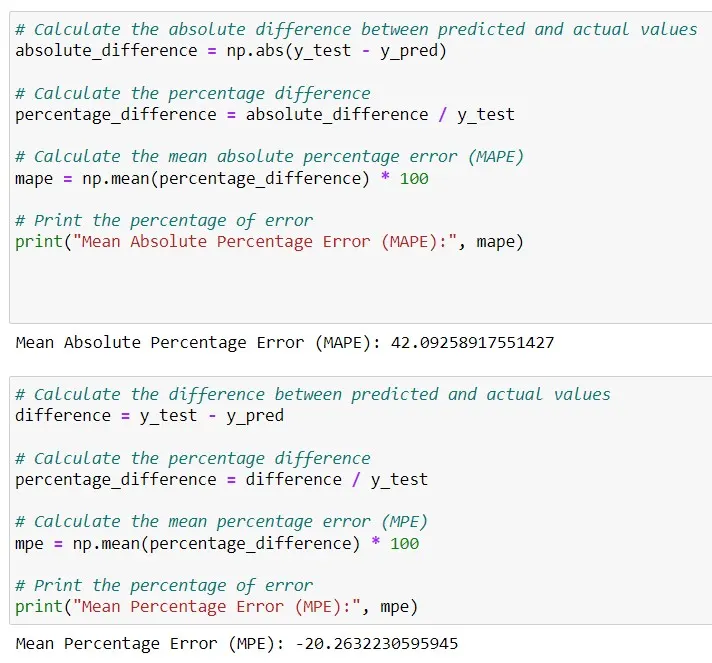
10. Give the percentage of error in regression model.
<!--[endif]-->
11. Give the 95% confidence interval for average charge insurance.
import numpy as np
from scipy.stats import t
# Define the insurance charges dataset
charges = df['charges']
# Calculate the sample mean and sample standard deviation
x_bar = np.mean(charges)
s = np.std(charges, ddof=1)
# Calculate the sample size
n = len(charges)
# Calculate the critical value (t) for the desired confidence level and degrees of freedom
confidence_level = 0.95
df = n - 1
t_value = t.ppf(confidence_level, df)
# Calculate the standard error
SE = s / np.sqrt(n)
# Calculate the margin of error
ME = t_value * SE
# Calculate the lower and upper bounds of the confidence interval
LB = x_bar - ME
UB = x_bar + ME
# Print the confidence interval
print("95% Confidence Interval for Average Charge Insurance:")
print("Lower Bound:", LB)
print("Upper Bound:", UB)

<!--[endif]-->