Project 1

Project 1: Development of Hybrid Drives using MATLAB & Simulink

Aim

The task of this project is to compute the fuel economy numbers for the given vehicle (kmpl) on the urban cycle (UDDS) and highway cycle (HWFET). Also, to analyze and understand the vehicle operating points in terms of engine speed, torque, transmission speeds, pedal positions, gear, distance traveled, etc.

Objectives

• Compute the fuel efficiency numbers (kmpl) for the UDDS and HWFET cycles.

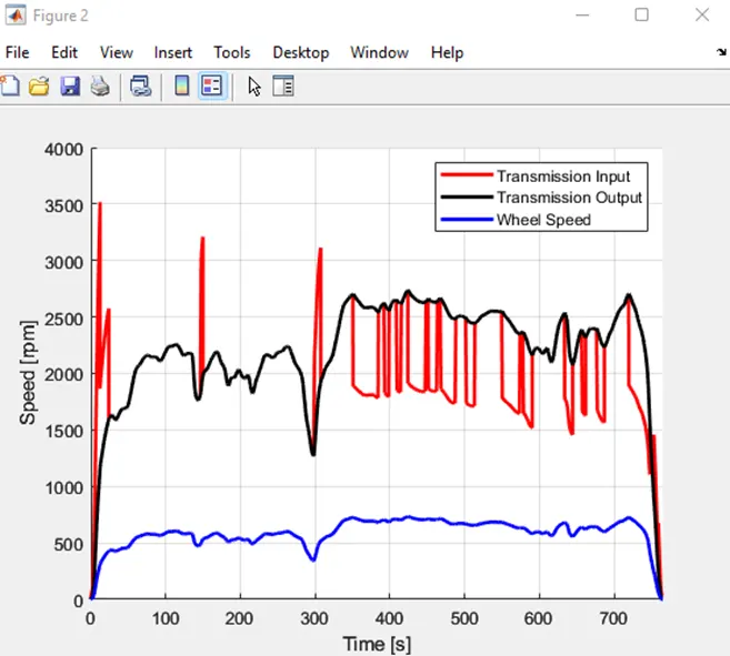
• Create a single plot with the time traces for the engine, transmission input, transmission output, and wheel speed.

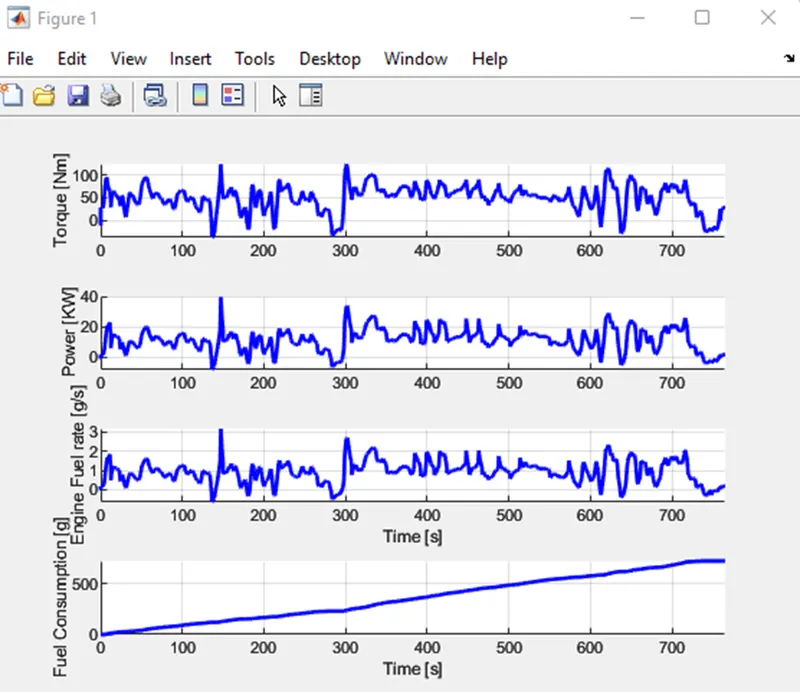
• Use subplots to plot engine torque, power, fuel rate, and power, fuel rate, and fuel consumption.

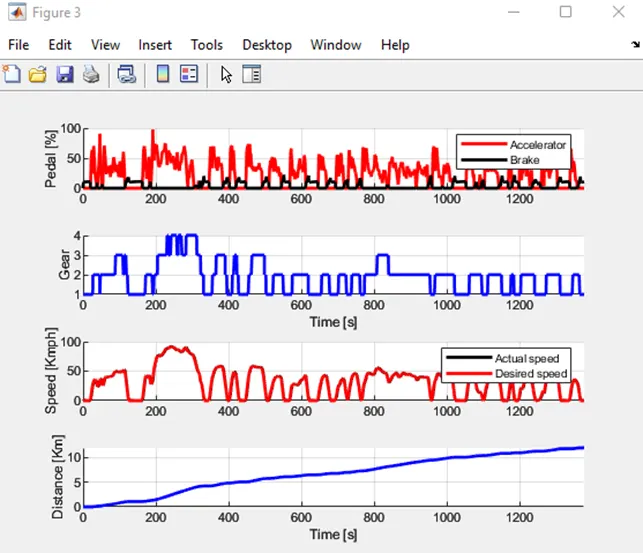
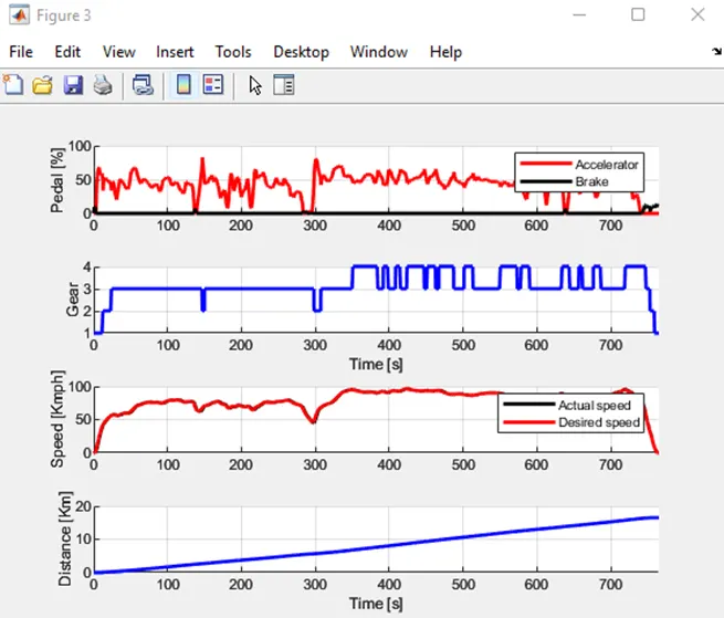
• Use subplots to map the accelerator and brake pedals, gear command, desired and actual vehicle speeds, and vehicle distance.

• Use subplots to map the accelerator and brake pedals, gear command, desired and actual vehicle speeds, and vehicle distance.

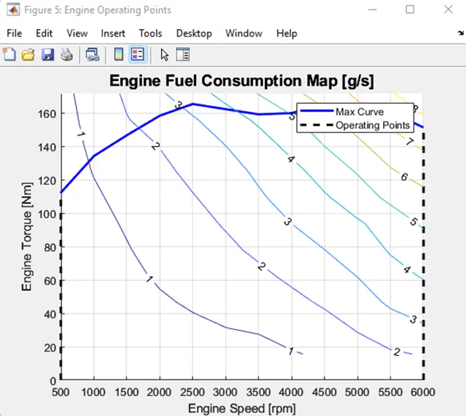
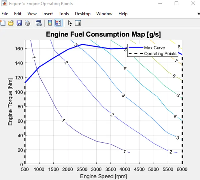
• On the engine fuel map, plot the engine operating points.

• On each of these plots, jot down suitable, succinct remarks describing how the vehicles behaved during the drive cycle. Plots should be created for both drive cycles

Theory

Forward Modelling Approach

• The engine-to-wheel, rear-to-front, and cause-and-effect methods are other names for the forward modeling methodology. Calculation flows from engine to wheel in the same direction as positive power flow.
• This method is based on equations for vehicle dynamics, the behavior of individual powertrain parts, and their dynamic interplay.
• Moreover, a driver controller is necessary to set the calculation start time and operate the vehicle to follow a chosen speed. The controller is set up to simulate how the driver will operate the brakes or the accelerator to match the intended speed, allowing for the study of driver behavior. The controller is utilized as a feedback loop component to calculate the energy necessary to power the vehicle.

Estimation Models of Energy Consumption for the Vehicle

Models for Predicting Automotive Energy Consumption. Three broad categories can be used to classify energy consumption estimation models:

Analytical models: By building a vehicle model in MATLAB/Simulink, analytical models may be constructed that is indicative of the behavior of the vehicle. Key theoretical equations serve as their foundation. Based on vehicle dynamics theory, a model of the vehicle's dynamics is constructed to determine the amount of power needed at the wheels to overcome the aerodynamic drag, rolling resistance, inertia, gradient, and transmission resistances. The necessary power is derived from the tractive force, which is expressed as the total of the aforementioned resistance forces.

Statistical models: In order to determine the empirical links between the various aspects affecting a vehicle's energy usage, statistical models are developed based on real-world driving data analysis.

Computational models: The two basic categories of computational models for estimating energy usage are: Models based on Artificial Neural Networks (ANN). Models based on clustering.

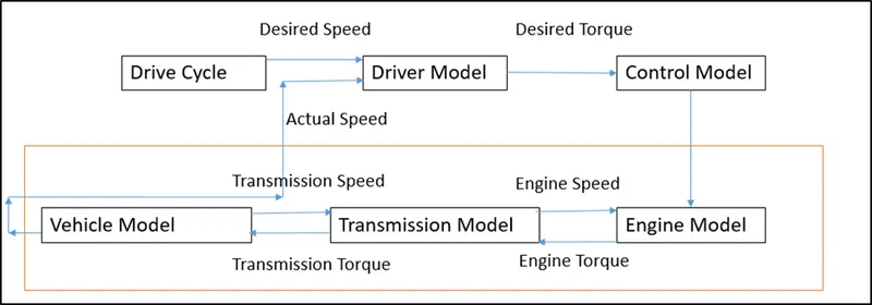
Figure 1 presents the architecture of the forward conventional vehicle model.

• This model has a driver model that, depending on the drive cycle and the actual speed of the vehicle, sends input commands for acceleration and brake torque.

• A control model that alters the gear command and manages brake torque in response to driver input while controlling engine torque to the appropriate range.

• The transmission model provides the driver model with feedback about the vehicle's actual speed. The engine, transmission, differential, wheel, and vehicle dynamics models are all included independently in the model.

Vehicle Model

To load every variable required to run and post-process the Simulink model, a MATLAB script has been written. From here, the drive cycle selection is also made. The script is started in MATLAB to load all the variables in the workspace before running the Simulink vehicle model.

Matlab Code (Script File)

%%%%%%%%%%%%%%%%%%%%%%%%%%%%%%%%%%%%%%%%%%%%%%%%%%%%%%%%%%%%%%%%%%%%%

%% Skill-Lync -> Hybrid Drives Development

% Project 1 - Conventional Vehicle Model

% By - Abdellatif Sadeq

% Description:

%% Initialization File

% Initialization file for loading the variables for the Conventional vehicle simulation model

%% Vehicle Parameters

M = 1500; % Vehicle weight [kg]

Cr = 0.015; % Rolling resistance coefficient

Rw = 0.35; % Rolling radius [m]

Cd = 0.33; % Drag coefficient

Af = 2; % Frontal area [m2]

rhoa = 1.225; % Air density [kg/m3]

Vwind = 0; % Wind velocity [kmph]

g = 9.81; % Gravitational acceleration [m/s2]

theta = 0; % Slope [deg]

myu_road_tire = 1; % Coefficient of friction between tire - road interface

%% Powertrain Parameters

FDR = 3.73; % Final Drive Ratio / Diff Ratio

DiffEff = 0.99; % Differential efficiency (assumed independent of operating conditions)

NumGear = 4; % Number of gears in transmission

TransGear = [1:NumGear]; % Transmission Gears

TransRatio = [3.06, 1.62, 1, 0.7]; % Corresponding Transmission ratios

TransEff = 0.90; % Transmission efficiency (assumed independent of operating conditions)

TC_SR = [0, .5, .6, .7, .8, .87, .92, .94, .96, .97, 1]; % Torque Converter Speed Ratio (Matlab default) -> TurbSpd/PumpSpd

TC_TR = [2.232, 1.5462, 1.4058, 1.2746, 1.1528, 1.0732, 1.0192, 1, 1, 1, 1]; % Torque Converter Torque Ratio (Matlab default) -> TurbTrq/PumpTrq

TC_Cf = 1e-4 * [.72558, .66322, .63463, .59042, .51331, .4144, .29287, .22444, .12186, .04386, 0]; % Torque Converter Capacity Factor (Matlab default) -> PumpTrq/PumpSpd^2 [Nm/rpm^2]

load Vehicle_Data/Engine_data_1_9L_Saturn_95kW

load Vehicle_Data/Trans_Shift_map

%% Driver Parameters

Kp = 10; % P gain for driver PI model

Ki = 1; % I gain for driver PI model

Drive_Cycle_Select = 1; % Drive cycle selection

% Drive cycle values in m/s

if Drive_Cycle_Select == 1

load DriveCycles/UDDS;

elseif Drive_Cycle_Select == 2

load DriveCycles/HWFET;

elseif Drive_Cycle_Select == 3

load DriveCycles/FTP;

elseif Drive_Cycle_Select == 4

load DriveCycles/US06;

elseif Drive_Cycle_Select == 5

load DriveCycles/NEDC;

elseif Drive_Cycle_Select == 6

load DriveCycles/WLTP;

end

time_end = cyc_time(end);

vel_end = cyc_vel(end);

Simulink Model

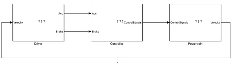
• The driver model, control model, and powertrain block are the three basic subblocks used to build the convection model in Simulink.

• The controller block sends control signals for engine torque, gear shifting, and brake torque to the Powertrain model while the driver block receives feedback on the actual vehicle speed and supplies the controller block with the necessary acceleration or braking output.

Driver Model

A fundamental PI controller called Driver Model produces outputs from the accelerator and brake pedals that are matched to the desired and actual vehicle speeds.

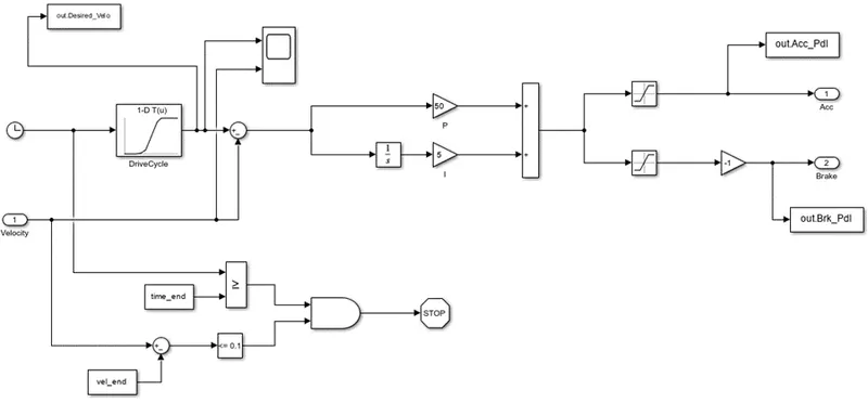
By giving the controller output for the accelerator and brake pedals, the PI controller manages the discrepancy between the needed driving cycle and the actual vehicle speed.

Controller Model

The 'Controller' block, which stands in for the electronic control systems, is the brain of the car. It produces the required engine torque, desired gearbox gear, and desired brake torque based on the driver's inputs. These inputs are supplied to the "Powertrain" block, which reflects the vehicle's drivetrain.

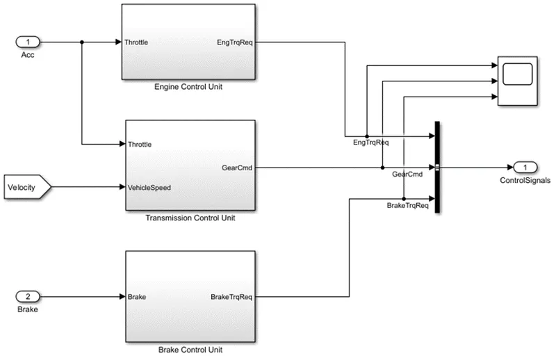
• An engine control unit, a transmission control unit, and a brake control unit make up the controller.
• You can scope any control signal.

Engine Control Unit

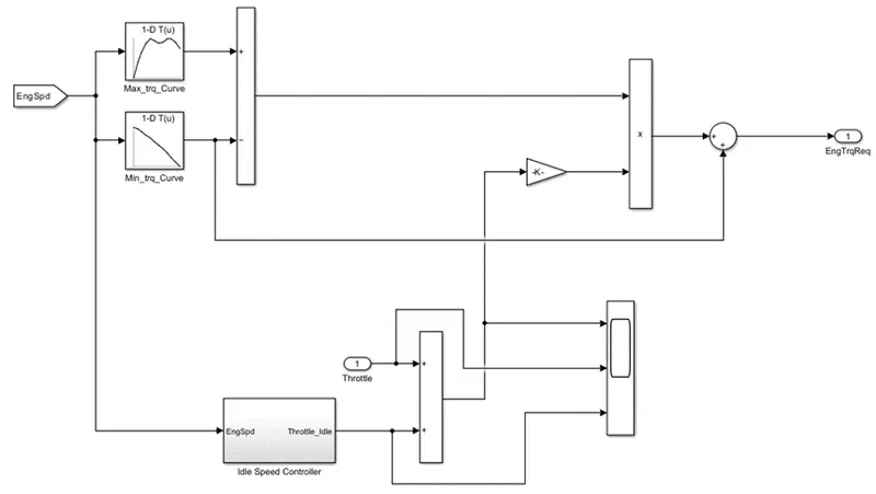
Idle Speed Controller

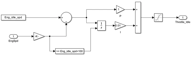
The engine management system gives the engine block the necessary torque command by comparing engine speed to the lookup table's maximum and lowest torque curves. To estimate the torque input needed for the engine, the throttle input is combined with the idle speed throttle and gains with the torque output from the lookup table.

This block can be used to scope throttle input, idle throttle, and their sum.

Transmission Control Block

• The study flow variable chart is used by the transmission control block to regulate gear shifting.

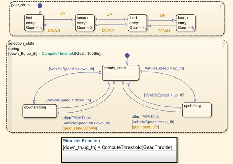
• The throttle input and vehicle speed are used to control gear changing.

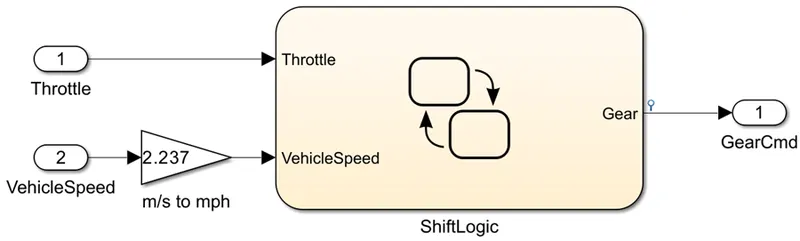
• The Transmission block receives the gear command, which it uses to choose the preferred gear ratio.

Brake Control Unit

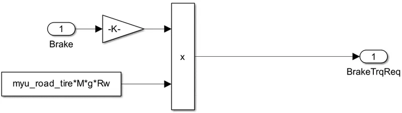
The brake controller generates the necessary brake torque in accordance with the input from the brake pedal, then transmits that torque to the wheel block in the transmission model.

Powertrain Model

All the parts that transform an engine's power into motion are included in the powertrain model.

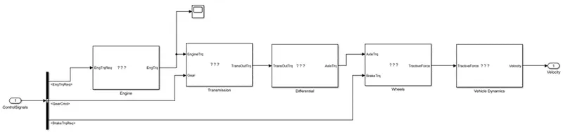
This covers the subsystems for the vehicle's engine, transmission, differential, wheels, and body dynamics.

Engine Model

• Depending on Engine speed the controller's necessary torque reaches saturation between the maximum and minimum torque curves and transfers engine torque to the transmission block.
• Based on engine speed and torque, the fuel flow rate is calculated using a 2D lookup table. The fuel consumption is then calculated using an integration of the fuel flow rate.
• The “To workspace” block is used to send estimated values for fuel flow rate, fuel consumption, engine torque, and engine speed to the MATLAB workspace.
• Fuel consumption and engine fuel flow rate are scoped.

Transmission Model

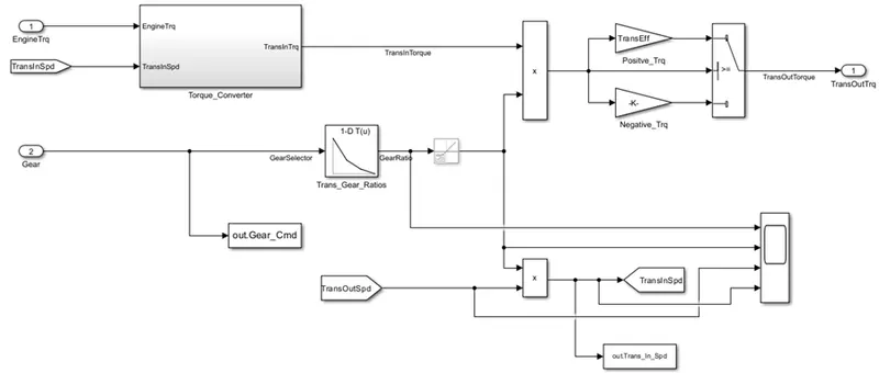
A torque converter links the engine block to the automatic transmission. The differential is connected to the transmission's output.

Torque Converter

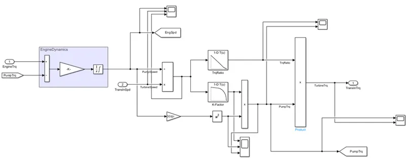
In this block, the engine torque is multiplied by the transmission control unit's gear selection, and the torque converter's efficiency and engine dynamics are taken into account.

Differential Model

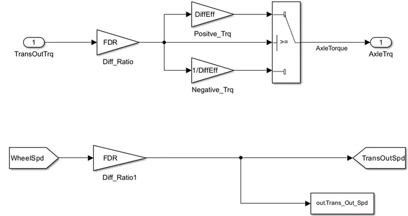
In this block, the differential ratio and differential efficiency are multiplied by the transmission output torque to produce the axle torque, which is then transmitted to the wheel.

Wheel Model

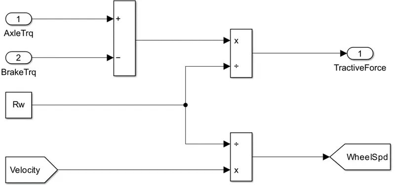
• To calculate the tractive force, the axle torque from the control model is subtracted from the brake torque, which is then divided by the rolling radius.
• The vehicle velocity is used to calculate the Wheel speed, which is then saved in the workspace.

Vehicle Dynamics

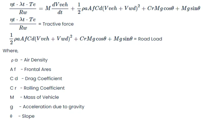
The "Vehicle Dynamics" block displays the vehicle's longitudinal dynamics as well as the road load.

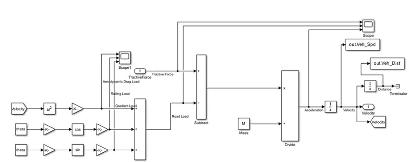
• To determine the vehicle's speed, Tractive Force and Road Loads are used.

• MATLAB Script is used to load the variables onto the workspace.

• Calculations are made and kept in the workspace for the Acceleration, Velocity, and Distance traveled.

Simulation Results

• UDDS Drive Cycle

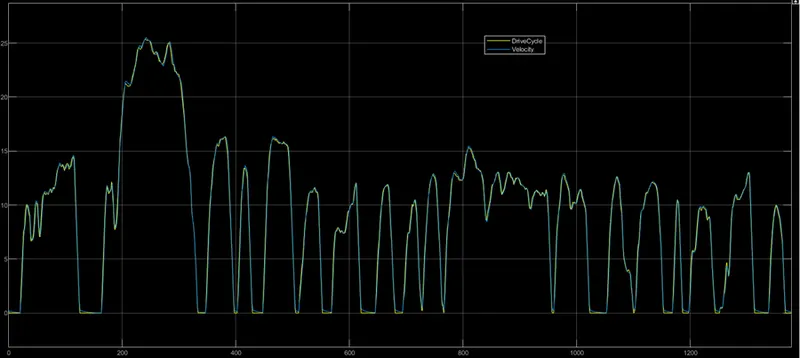
Drive Cycle and Velocity

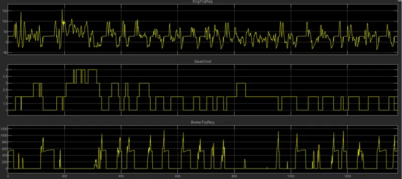
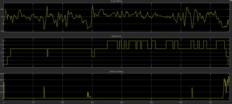
Control Signals (Engine Torque Request, Transmission Gear, and Brake Torque Request)

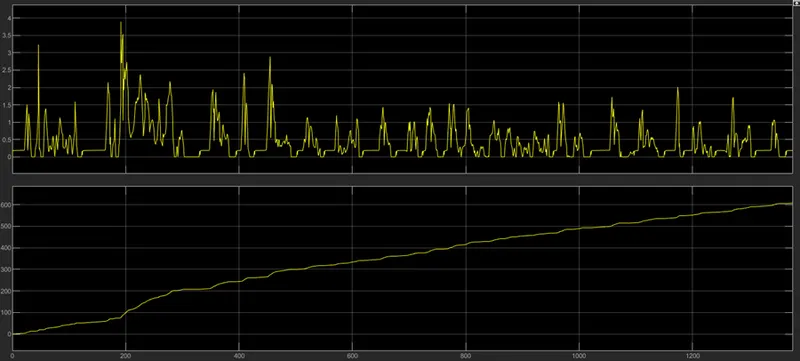
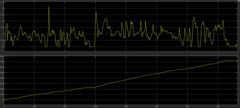
Engine Fuel Flow Rate and Consumption

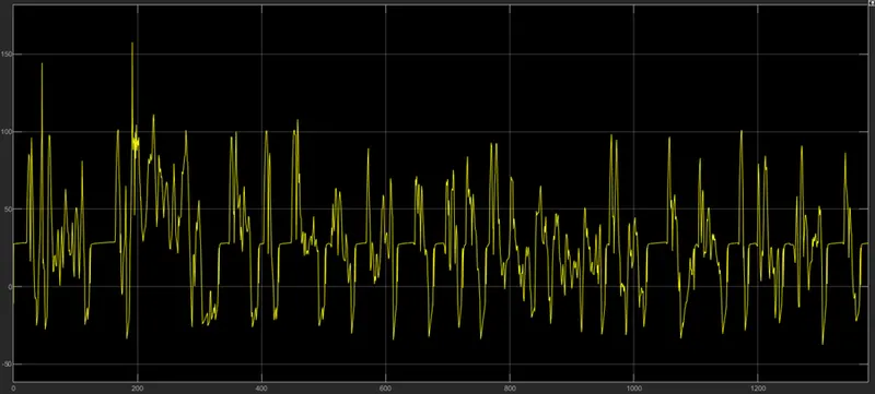
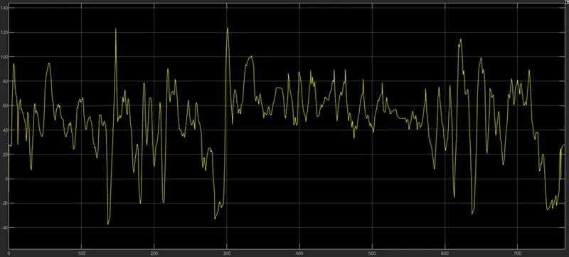
Engine Torque

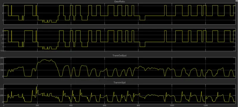
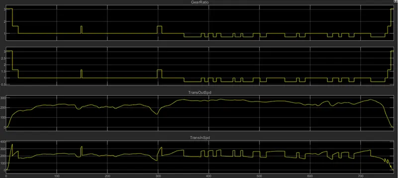
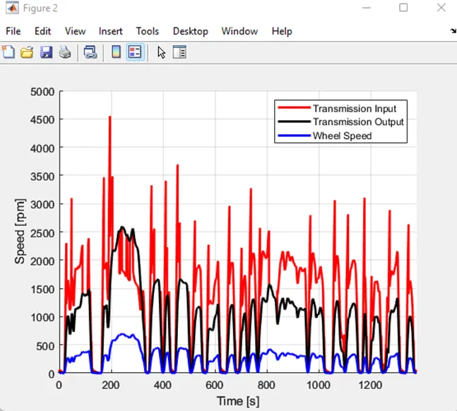
Gear Ratio, Transmission Output, and Input Speeds

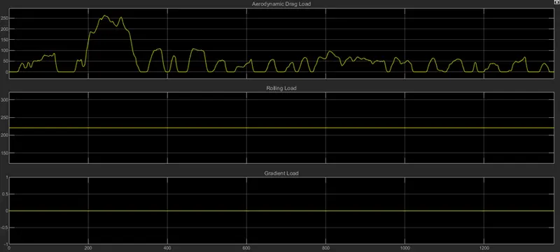
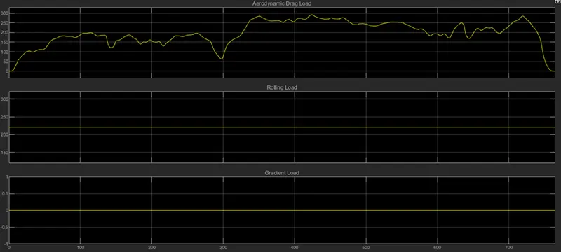
Road Loads (Aerodynamic Road Load, Rolling Load, and Gradient Load)

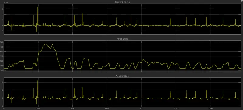
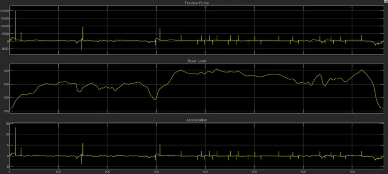
Tractive Force, Road Load and Acceleration

• HWFET Drive Cycle

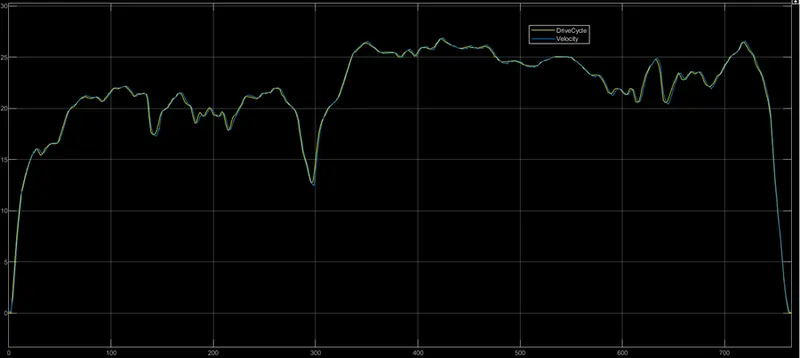
Drive Cycle and Velocity

Control Signals (Engine Torque Request, Transmission Gear, and Brake Torque Request)

Engine Fuel Flow Rate and Consumption

Engine Torque

Gear Ratio, Transmission Output, and Input Speeds

Road Loads (Aerodynamic Road Load, Rolling Load, and Gradient Load)

Tractive Force, Road Load and Acceleration

Post-Processing

To analyze data and create charts, a MATLAB script is written. Here, we rename the model-loaded variables, perform some elementary post-processing computations, and provide results and visualizations.

%%%%%%%%%%%%%%%%%%%%%%%%%%%%%%%%%%%%%%%%%%%%%%%%%%%%%%%%%%%%%%%%%%%%%

%% Skill-Lync -> Hybrid Drives Development

% Project 1 - Conventional Vehicle Model

% By - Abdellatif Sadeq

%% Post-Processing File

% File for post-processing the Conventional vehicle simulation model data

%% Renaming variables

Time = out.tout;

Acc_Pdl = out.Acc_Pdl; % Accelerator pedal [%]

Brk_Pdl = out.Brk_Pdl; % Brake pedal [%]

Gear_Cmd = out.Gear_Cmd; % Transmission gear

Trans_In_Spd = out.Trans_In_Spd*30/pi; % Transmission input speed [rpm]

Trans_Out_Spd = out.Trans_Out_Spd*30/pi;% Transmission output speed [rpm]

Eng_Trq = out.Eng_Trq; % Engine brake torque [Nm]

Eng_Spd = out.Eng_Spd*30/pi; % Engine speed [rpm]

Eng_Fuel_rate = out.Eng_Fuel_Rate; % Engine Fuel Rate [gkW]

Eng_Fuel_Consump = out.Eng_Fuel_Consumption; % Engine fuel consumption [g]

Veh_Dist = out.Veh_Dist/1000; % Distance traveled by vehicle [km]

Veh_Spd = out.Veh_Spd*18/5; % Vehicle speed [kmph]

Whl_Spd = out.Whl_spd*30/pi; % Wheel speed [rpm]

Desired_spd = out.Desired_Velo*18/5; % Desired Speed [Kmph]

%% Data Analysis

Eng_Pwr = Eng_Spd.*pi/30.*Eng_Trq/1000; % Engine brake power [kW]

rho_petrol = 0.7197; % Density of petrol [kg/L]

kmpl = Veh_Dist(end)/(Eng_Fuel_Consump(end)/1000/rho_petrol); % Fuel economy [kmpl]

% Display Fuel Economy of the Cycle

fprintf('nFuel Economy = %2.2fKmplnn',kmpl);

%% Plotting vehicle characteristics time trace

% Plotting engine torque, engine power, fuel rate and fuel consumption

figure(1)

subplot(4,1,1)

hold on

grid on

plot(Time, Eng_Trq, 'linewidth', 2, 'Color', 'blue');

ylabel('Torque [Nm]')

xlim([0, Time(end)]);

subplot(4,1,2)

hold on

grid on

plot(Time, Eng_Pwr, 'linewidth', 2, 'Color', 'blue');

ylabel('Power [KW]')

xlim([0, Time(end)]);

subplot(4,1,3)

hold on

grid on

plot(Time, Eng_Fuel_rate, 'linewidth', 2, 'Color', 'blue');

xlim([0, Time(end)]);

xlabel('Time [s]');

ylabel('Engine Fuel rate');

subplot(4,1,4)

hold on

grid on

plot(Time, Eng_Fuel_Consump, 'linewidth', 2, 'Color', 'blue');

xlim([0, Time(end)]);

xlabel('Time [s]');

ylabel('Fuel Consumption [g]');

% Plotting transmission input, output and wheel speeds

figure(2)

hold on

grid on

plot(Time, Trans_In_Spd, 'linewidth', 2, 'Color', 'red');

plot(Time, Trans_Out_Spd, 'linewidth', 2, 'Color', 'black');

plot(Time, Whl_Spd, 'linewidth', 2, 'Color', 'blue');

xlabel('Time [s]')

ylabel('Speed [rpm]')

xlim([0, Time(end)]);

legend('Transmission Input','Transmission Output','Wheel Speed');

%Plotting accelerator and brake pedal gear command, vehicle desired and actual speed, vehicle distance

figure(3)

subplot(4,1,1)

hold on

grid on

plot(Time, Acc_Pdl, 'linewidth', 2, 'Color', 'red');

plot(Time, Brk_Pdl, 'linewidth', 2, 'Color', 'black');

ylabel('Pedal [%]')

xlim([0, Time(end)]);

legend('Accelerator','Brake');

subplot(4,1,2)

hold on

grid on

plot(Time, Gear_Cmd, 'linewidth', 2, 'Color', 'blue');

xlim([0, Time(end)]);

xlabel('Time [s]');

ylabel('Gear');

subplot(4,1,3)

hold on

grid on

plot(Time, Veh_Spd, 'linewidth', 2, 'Color', 'black');

plot(Time, Desired_spd, 'linewidth', 2, 'Color', 'red');

ylabel('Speed [Kmph]')

xlim([0, Time(end)]);

legend('Actual speed','Desired speed');

subplot(4,1,4)

hold on

grid on

plot(Time, Veh_Dist, 'linewidth', 2, 'Color', 'blue');

xlim([0, Time(end)]);

xlabel('Time [s]');

ylabel('Distance [Km]');

%% Plotting Drive Cycle

figure(4)

hold on

grid on

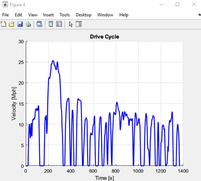
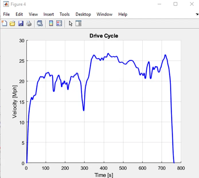
plot(cyc_time, cyc_vel, 'linewidth', 2, 'Color', 'blue');

xlabel('Time [s]')

ylabel('Velocity [Mph]')

title('Drive Cycle')

% Test Results

Avg_speed = sum(Veh_Spd)/length(Veh_Spd);

Max_Speed = maxk(Veh_Spd,1);

table(Avg_speed,Max_Speed,kmpl,'VariableNames',{'Average Speed [kmph]','Maximum Speed [kmph]','Fuel Economy [kmpl]'})

%% Plotting engine operating points on engine fuel map

figure('Name','Engine Operating Points');

hold on

grid on

title('Engine Operating Points','fontsize',14);

p1=plot(Eng_map_spd*30/pi,Eng_max_trq,'linewidth',2,'color','b');

p2=line([Eng_map_spd(end)*30/pi Eng_map_spd(end)*30/pi],[0 Eng_max_trq(end)]);

set(p2,'linewidth',2,'linestyle','--','color','k');

p3=line([Eng_map_spd(1)*30/pi Eng_map_spd(1)*30/pi],[0 Eng_max_trq(1)]);

set(p3,'linewidth',2,'linestyle','--','color','k');

[c,h] = contour(Eng_map_spd'*30/pi,Eng_map_trq,Eng_fuel_map');

clabel(c,h);

xlabel('Engine Speed [rpm]');

ylabel('Engine Torque [Nm]');

title('Engine Fuel Consumption Map [g/s]');

legend([p1 p3],{'Max Curve','Operating Points'});

axis([Eng_map_spd(1)*30/pi Eng_map_spd(end)*30/pi 0 Eng_map_trq(end)]);

Results

• UDDS Cycle

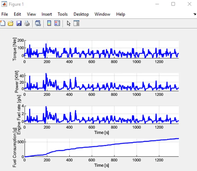
Engine Torque, Engine Power, Fuel Flow Rate and Fuel Consumption

Transmission Input, Output, and Wheel Speeds

Accelerator and Brake Pedal Gear Command, Vehicle Desired and Actual Speeds, and Vehicle Distance

Drive Cycle

Engine Operating Points on Engine Fuel Map

• HWFET Cycle

Engine Torque, Engine Power, Fuel Flow Rate and Fuel Consumption

Transmission Input, Output, and Wheel Speeds

Accelerator and Brake Pedal Gear Command, Vehicle Desired and Actual Speeds, and Vehicle Distance

Drive Cycle

Engine Operating Points on Engine Fuel Map

Average and Maximum Speeds, and Fuel Economy Number (kmpl)

UDDS Drive Cycle

HWFET Drive Cycle

Observations

• Since there is less brake pedal contact and idle time during the UDDS drive cycle, the city fuel economy is significantly lower than the HWFET drive cycle.

• The torque converter contributes significantly to the input speed variation, and the transmission input speed varies in response to the engine torque required to complete the driving cycle.

• Differential and gear ratios affect wheel speed and transmission output speed.

• Different driving cycles have varied torque requirements, which affect the fuel flow rate and how much fuel is used.

• Since the UDDS drive cycle is not very smooth and gear shifts are required frequently, the accelerator and brake pedals are utilized more frequently.

• On the highway drive cycle, there are fewer brake requirements, more accelerator pedals are depressed, and gear transfers happen more frequently.

• On the engine fuel consumption map, the engine operating points are shown, and the operating point is below the maximum torque curve for both cycles.