Plotting the PV Diagram for an Otto Cycle and Calculating its Thermal Efficiency

Objective: To write a program in MATLAB which can calculate the state properties at different states of the otto cycle and hence, plot the PV diagram. The program should also be able to display the thermal efficiency of the cycle.

Procedure:-

• We write a program in which based on the input and geometric parameters, the state properties like pressure, volume and temperature are calculated at different states of the otto cycle.
• By using these state properties, the PV diagram is plotted.
• Finally, the thermal efficiency of the engine is evaluated using the temperature values. We know, the thermal efficiency,
  • `eta = 1 - frac{Q_c}{Q_h}` where `Q_c`is the heat dissipated to the environment and `Q_h`is the heat supplied through the spark plug.
  • But we know that `Q_c = mc_v(T_4 - T_1)` and `Q_h = mc_v(T_3 - T_2)`.
  • Therefore, `eta = 1 - frac{T_4 - T_1}{T_3 - T_2}`
• The code along with the explanation of different steps has been described below:
  • We defined a function named "engine_kinematics" in a seperate file. Its code is:-

  • % Defining a function which returns the values of volume and pressure at different points on the adiabatic process line
    function V = engine_kinematics(bore,stroke,con_rod,cr,start_crank,end_crank)
    	%Engine kinematics
    
    	% Geometric parameters
    	a = stroke/2;
    	R = con_rod/a;
    
    	% Volume parameters
    
    	% Stroke volume
    	V_s = pi*(1/4)*bore^2*stroke;
    	% Clearance volume
    	V_c = V_s/(cr - 1);
    
    	% Converting the start_crank and end_crank angles to radians
    	sc = deg2rad(start_crank);
    	ec = deg2rad(end_crank);
    
    	% Calculating volume and pressure values at 25 different points on the adiabatic process line
    
    	num_values = 25;
    
    	dtheta = (ec - sc)/(num_values - 1);
    
    	V = [];
    
    	for i = 1:1:num_values
    		theta = sc + i*dtheta;
    		% Using the formula to evaluate volume using the crank angle and the geometric parameters
    		term1 = 0.5*(cr - 1);
    		term2 = R + 1 - cos(theta);
    		term3 = (R^2) - ((sin(theta))^2);
    		Volume = V_c*(1 + term1*(term2 - (term3^0.5)));
    		V(end+1) = Volume;
        end
        
    end

  • The main code is:-

  • % Otto cycle simulator
    
    % Main code file
    
    % The function engine_kinematics has been defined separately.
    
    % Inputs
    
    % Pressure: unit in Pascal
    % Lets take this pressure as atmospheric pressure which is 101325 Pa.
    p1 = 101325;
    % Temperature at state 1: unit in Kelvin
    % Lets take this temperature as 300 K
    t1 = 300;
    gamma = 1.4;
    % Temperature at state 3: unit in Kelvin
    % Lets take this temperature as 2500
    t3 = 2500;
    
    % Geometrical parameters
    % Lets take bore, stroke and connecting rod to be 0.14 m, 0.18 m and 0.25 m respectively.
    bore = 0.14;
    stroke = 0.18;
    % connecting rod
    con_rod = 0.25;
    % compression ratio: Lets take this as 9
    cr = 9;
    
    % Volume computation
    
    % stroke volume
    v_s = pi*(1/4)*(bore^2)*stroke;
    % clearance volume
    v_c = v_s/(cr - 1);
    v1 = v_c + v_s;
    
    % state point 2
    v2 = v_c;
    
    % p2v2^gamma = p1v1^gamma
    p2 = (p1*v1^gamma)/(v2^gamma);
    
    % p2v2/t2 = p1v1/t1 | p1v1/t1 = rhs | t2 = p2v2/rhs
    rhs = p1*v1/t1;
    t2 = p2*v2/rhs;
    
    % Volume and pressure at different points on the compression process line (State 1 -> State 2)
    V_compression = engine_kinematics(bore,stroke,con_rod,cr,180,360);
    
    P_compression = [];
    
    constant = p1*(v1^gamma);
    
    for j = 1:1:length(V_compression)
    	Pressure = constant/((V_compression(j))^gamma);
    	P_compression(end+1) = Pressure;
    end
    
    % state point 3
    v3 = v2;
    
    % p3v3/t3 = p2v2/t2 = rhs
    p3 = rhs*t3/v3;
    
    % state point 4
    v4 = v1;
    
    % p4v4^gamma = p3v3^gamma
    p4 = p3*(v3^gamma)/(v4^gamma);
    
    % p4v4/t4 = p3v3/t3 = rhs
    t4 = p4*v4/rhs;
    
    % Volume and pressure at different points on the expansion process line (State 3 -> State 4)
    
    V_expansion = engine_kinematics(bore,stroke,con_rod,cr,0,180);
    
    P_expansion = [];
    
    constant = p3*(v3^gamma);
    
    for k=1:1:length(V_expansion)
    	Pressure = constant/(V_expansion(k))^gamma;
    	P_expansion(end+1) = Pressure;
    end
    
    % Plotting each process line one by one
    
    % Adiabatic compression from state 1 to state 2
    plot(V_compression,P_compression)
    hold on
    % Isochoric process from state 2 to 3
    plot([v2,v3],[p2,p3])
    hold on
    % Adiabatic expansion process from state 3 to 4
    plot(V_expansion,P_expansion)
    hold on
    % Isochoric process from state 4 to 1
    plot([v4,v1],[p4,p1])
    xlabel('Volume (in m^3)')
    ylabel('Pressure (in Pa)')
    
    thermal_efficiency = 1 - ((t4 - t1)/(t3 - t2));
    print('The thermal efficiency of the otto cycle is:')
    disp("The thermal efficiency of the otto cycle is:-")
    disp(thermal_efficiency)

• Results:-
  

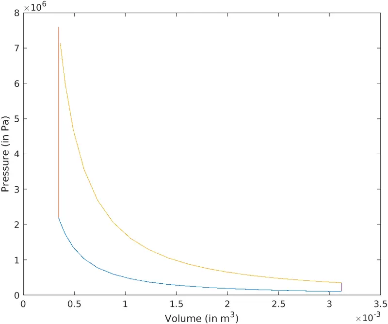
  • We get the PV diagram for the otto cycle:-
  • 
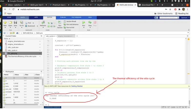
  • We also get the thermal efficiency of the otto cycle as can been seen in this screenshot:-
  • 

• Error Faced While Programming
  
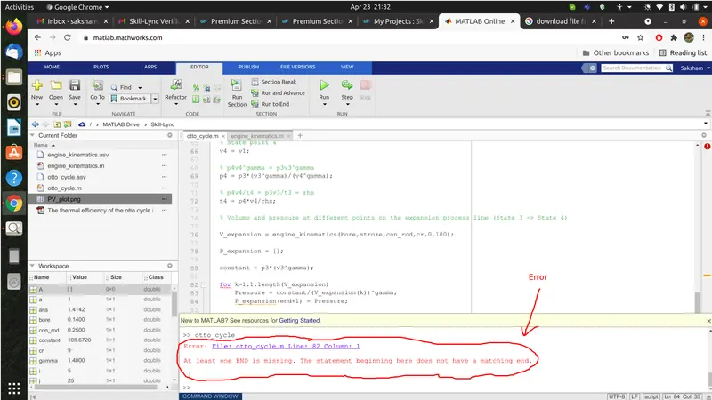
  • At one point, I got an error:-
    Error: File: otto_cycle.m Line: 82 Column: 1

    At least one END is missing. The statement beginning here does not have a matching end.

    An "end" was missing in the for loop. I added that to fix the error.

    Screenshot showing the error:-