Analysis of a PCB assembly for Conduction, Forced convection and Trace heating using Ansys Icepak

Introduction:

A printed circuit board (PCB) is generally a multi-layered board made of dielectric material and several layers of traces. From the thermal modeling point of view, a PCB may be treated as a homogeneous material with bi-directional thermal conductivity, i.e. thermal conductivity value is different in the normal-to-plane direction than that of in-plane. This approach is reasonable as long as the trace distribution is more-or-less uniform in any given layer. However, with the continuing challenges to increase product functionality while decreasing product size, designers are compelled to place more and more functionality on individual PCB's. As PCB's become more densely populated, their trace layers are becoming more non-uniform and it is prudent to use locally varying thermal conductivity information on the board.

Problem description:

A PCB board, library files and traces are imported to create the model. The model is solved for conduction only, without the components and then solved using the actual components with forced convection. Also, the model is analysed for trace heating.

Case-1: Conduction only model

A. Model creation:

Initially, the IDF file has been imported, where board and library files are loaded. A Reference image of the imported model has been attached below.

After Importing:

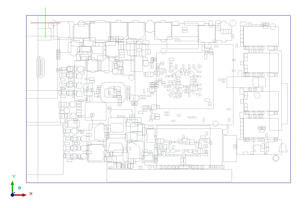
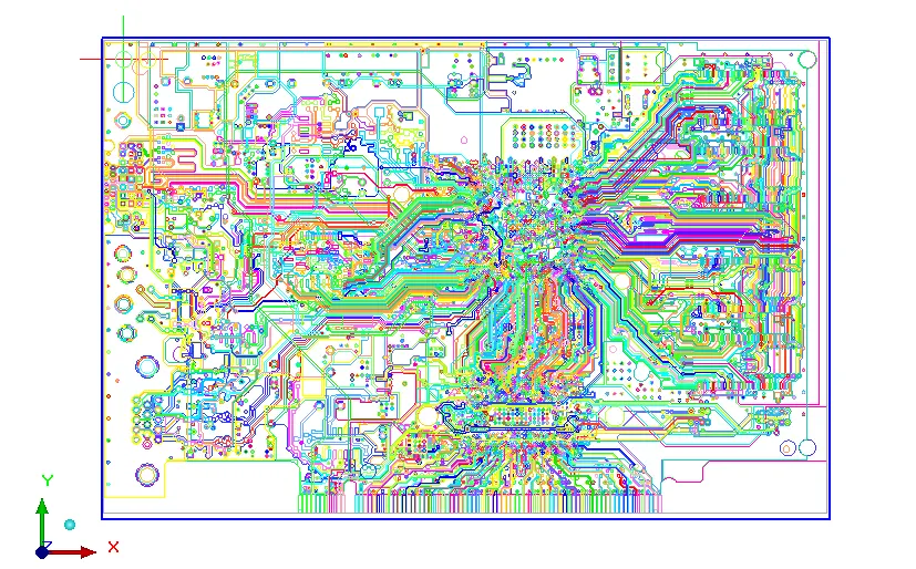
For conduction only model, all the components other than PCB is made inactive and trace file has been loaded by importing the pre-designed ECAD file.

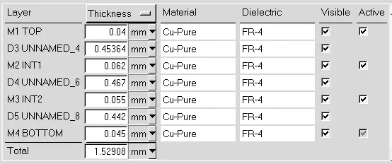
Boundary layer info:

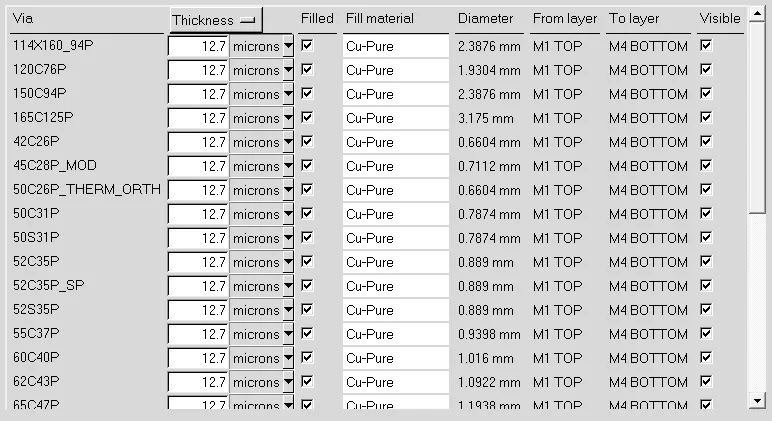
Vias info:

After importing trace layers:

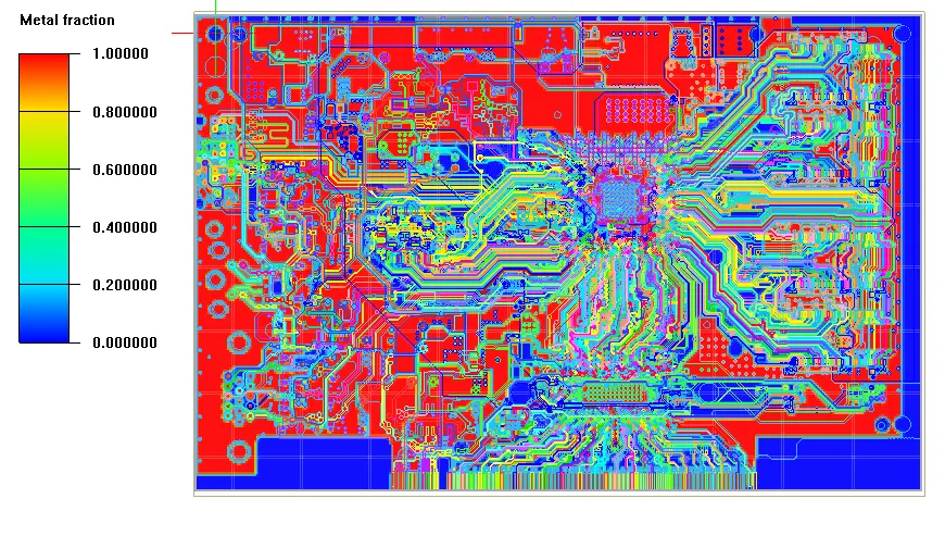
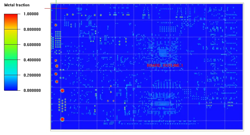
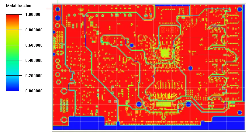
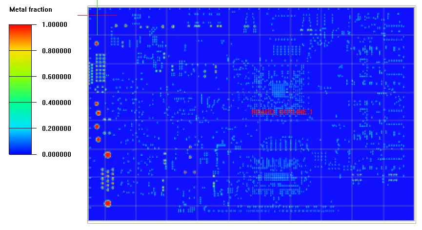
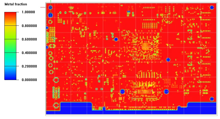
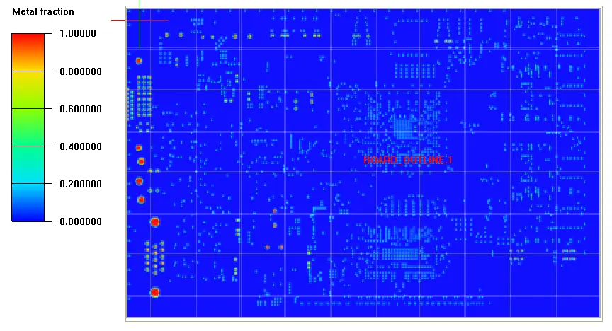
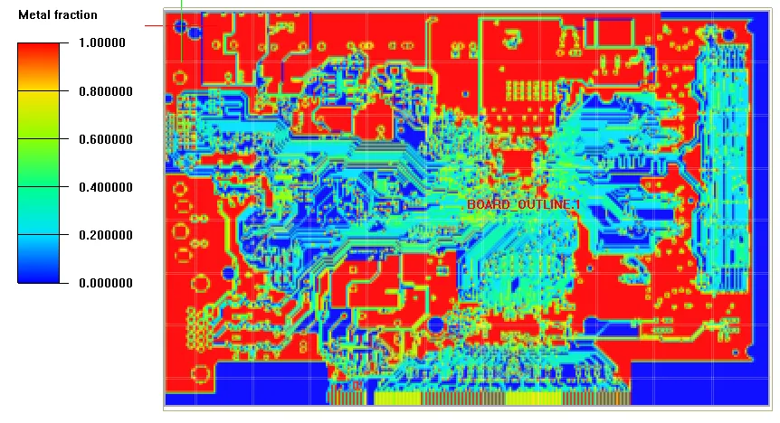
Metal fraction in all layers:

Layer-1:

Layer-2:

Layer-3:

Layer-4:

Layer-5:

Layer-6:

Layer-7:

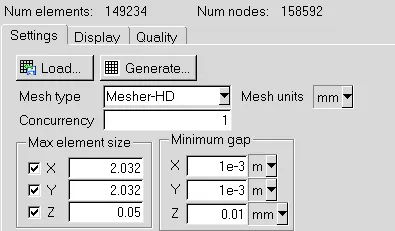
B. Mesh:

C. Setup:

I. Basic parameters:

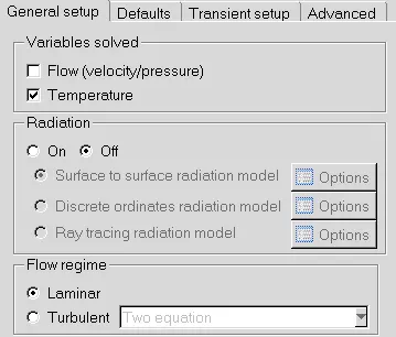
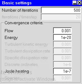
II. Basic settings:

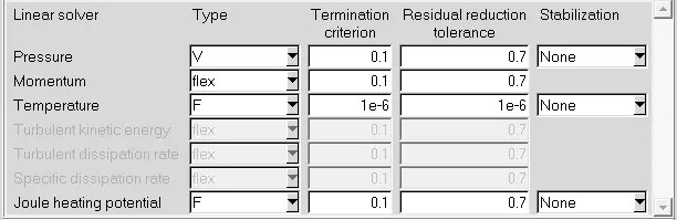
III. Advanced settings:

D. Solution description:

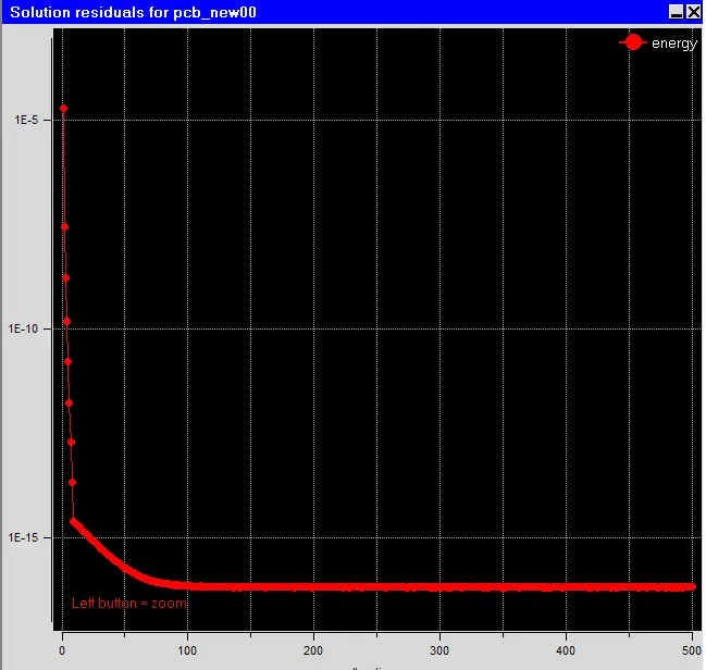
I. Residual plot

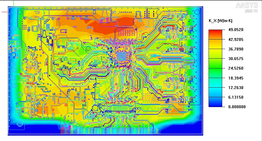
II. K_X distribution contour:

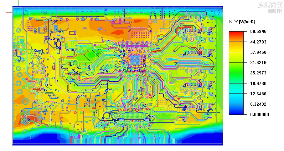
III. K_Y distribution contour:

Case-2: Convection model

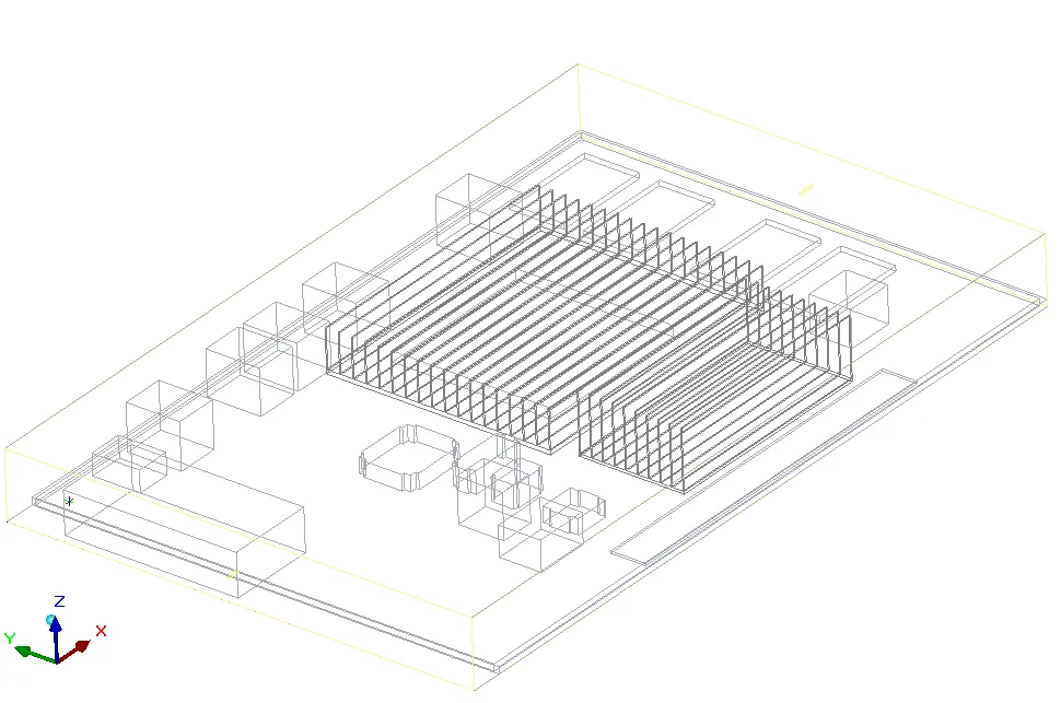
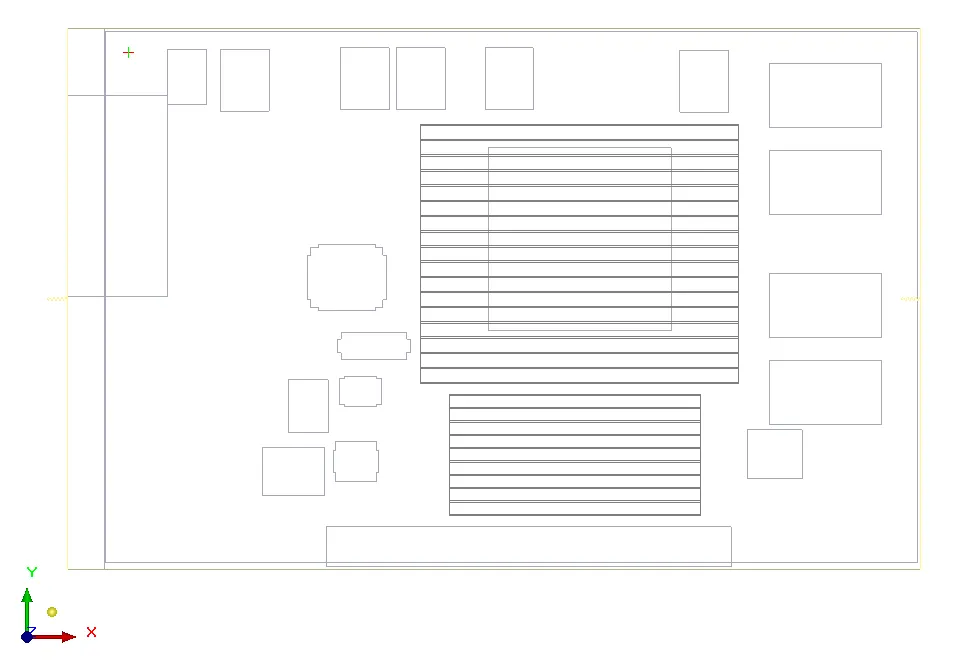
A. Cleaned-up model:

For the Forced convection, all the inactive components are activated again and cleanedup for proper analysis.

B. Mesh:

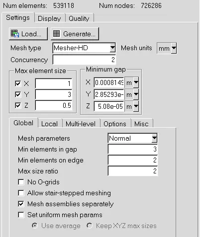
The General mesh settings used is provided below and the Heatsinks are clubed in an assembly and meshed separately without O-grids.

C. Setting up the case:

The Cabinet has been provided openings on min and max X sides and provided with a flow velocity. All the other sides are described as conductive walls.

Inlet velocity: 1.5m/s (Along -X)

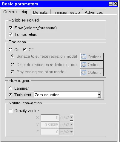
i. Basic parameters:

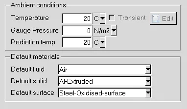
ii. Defaults:

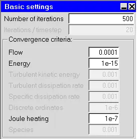
iii. Basic settings:

iv. Advanced settings:

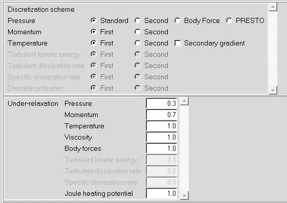
D. Solution description:

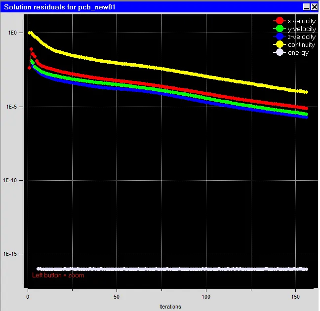
I. Residual plot:

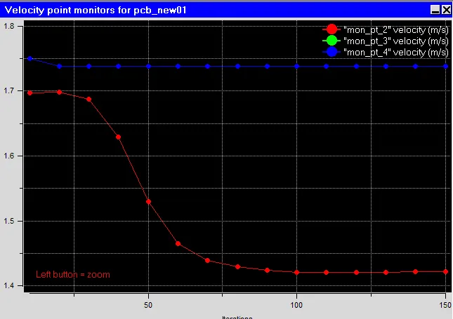
II. Monitor point velocity:

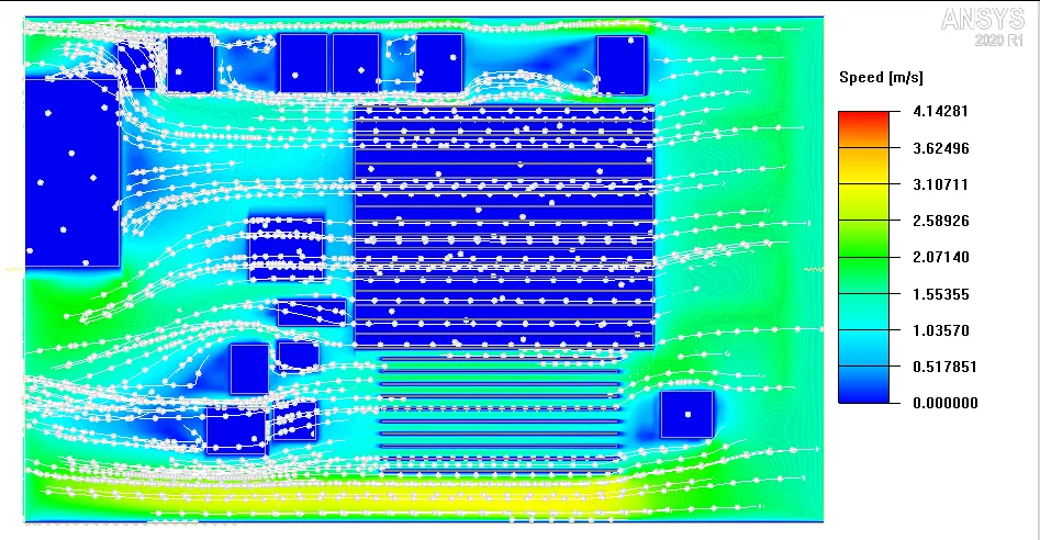
III. Velocity distribution:

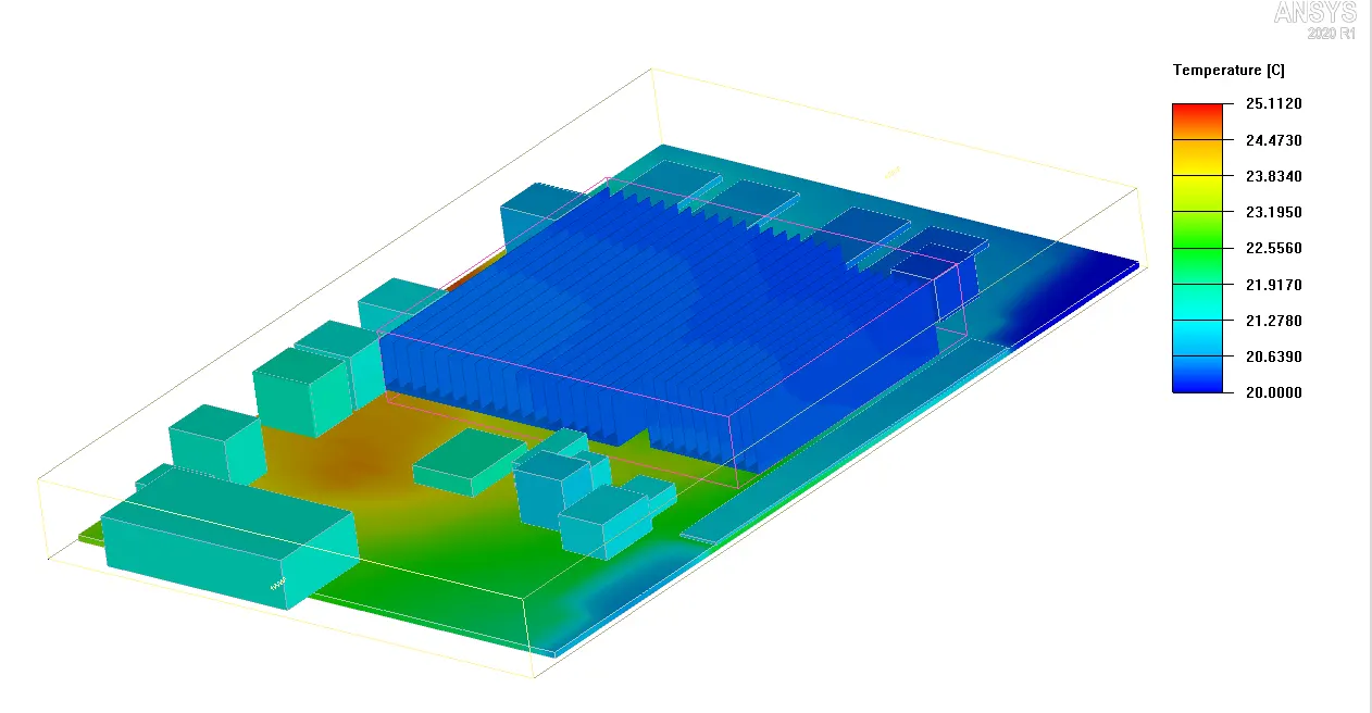
IV. Temperature distribution:

As there is no sources provided, the temperature over the domain remains the same (20 degC)

Case-3: Trace heating model

A. Trace creation and source addition:

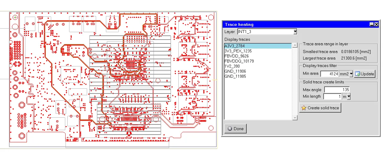
1. Build the Model – Edit the Board outline of the previous model to open the model trace heating panel. Select INT1_3 layer -> filter the trace to view by setting Min Area in the Display traces filter group box use a Min Area of 4124 mm2

2. Before you create a solid trace of trace A3V3_2261 set the Max angle filter to 135 and the Min length filter to 1.0 m to ignore the fine details in the trace geometry and reduce the mesh count.

3. Create a solid polygonal solid block for trace A3V3_2261

4. Select the polygonal trace just created from the Model manager window >> Under Thermal specification next to Joule heating, click Edit to open the Joule heating power panel. Set Resistivity, temperature coefficient (C), and reference temperature (Tref)

5. One source is for the current source (source.1) and the other for the voltage source (source.2)

Note:
Both sources are created at the same layer as the layer of the wire in. The area of each source is the area to apply the voltage or the current. The recommendation of the source objects pair for joule heating is the current-voltage pair or voltage- voltage pair.

Same setup and solution paramters as used for forced convection model is used and solved.

B. Solution description:

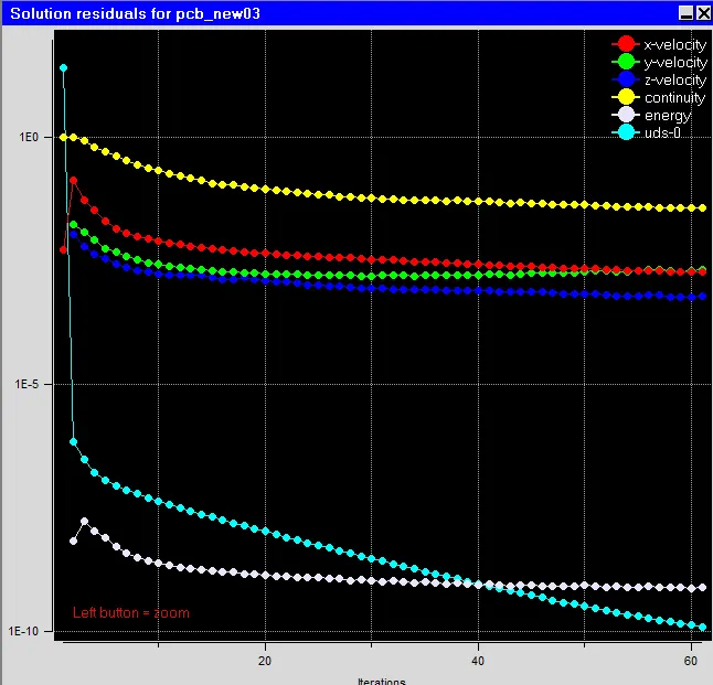
1. Residual plot:

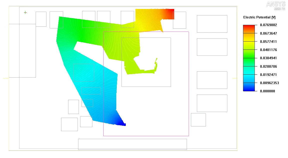
2. Electric potential contour:

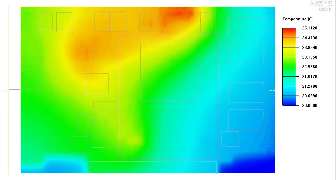
3. Temperature distribution:

The Flow of temperature from the positive current source to the neutral voltage source due to the potential difference created can be visualised in the provided contour plot.

Conclusion:

A PCB board's library files and traces are imported to create the model. The model is solved for conduction only, without the components and then solved using the actual components with forced convection. Also, the model is analysed for trace heating successfully.