Parsing NASA's Thermodynamic data using MATLAB

AIM: To parse the given file and perform the specified tasks using MATLAB.

EQUATION: The given formulae are as follows:

where;

`C_p` = Specific Heat (J/mol K)

`h` = Enthalpy (J)

`S` = Entropy (J/K)

`R` = Universal Gas Constant (J/mol K)

`T` = Temeprature (K)

OBJECTIVE:

1. To extract the 14 coefficients and calculate the enthalpy, entropy and specific heats for all the species in the data file.

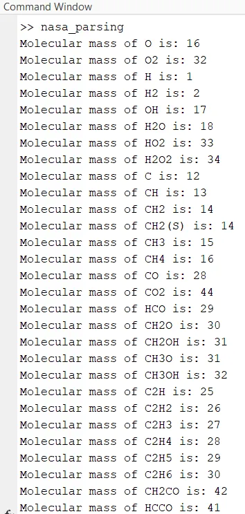
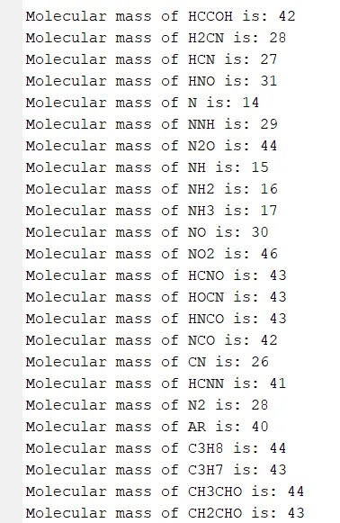
2. To calculate the molecular weight of each species and display it in the command window.

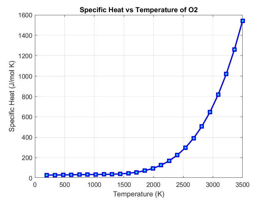
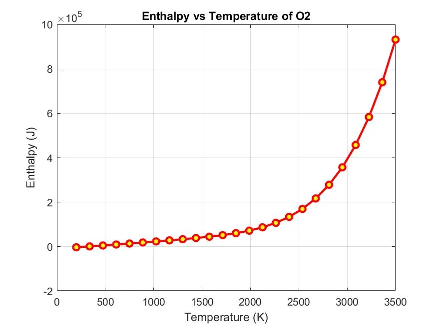
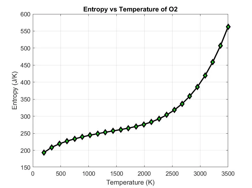
3. To plot the Specific Heat, Enthalpy and Entropy for the local temperature range (low temperature:high temperature) specific for each species.

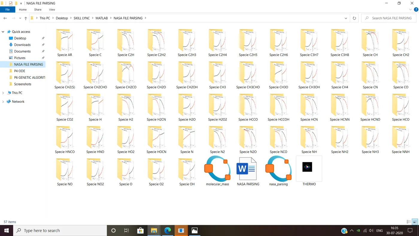
4. To save the plots as images with appropriate names and dump them in separate folders for each species with a suitable name. (All these should be generated automatically)

5. The main program should just take the THERMO.dat file as an input and generate Cp, h and S plots.

THEORY:

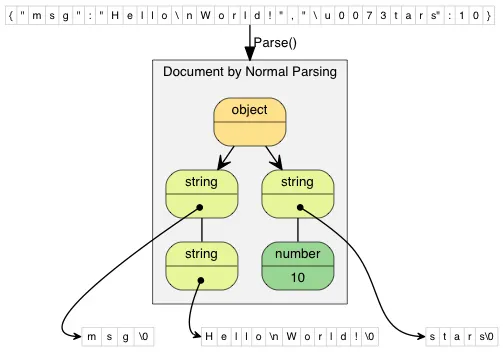
Parsing in computer languages refers to the syntactic analysis of the input code into its components parts in order to facilitate the writing of compilers and interpreters. It can be used to describe split or separation. Parsing a file means reading in a data stream of some sort and building an in-memory model of the semantic content of that data. This aims at facilitating performing some kind of transformation on the data. Specific Heat: The heat required to raise the temperature of the unit mass of a given substance by a given amount (usually one degree) is called Specific Heat Capacity. Enthalpy: It is equivalent to the total heat content of a system. It is equal to the internal energy of the system plus the product of pressure and volume. Entropy: It represents the unavailability of a system's thermal energy for conversion into mechanical work, often interpreted as the degree of disorder or randomness in the system. Molecular Mass: Molecular Mass Definition Molecular mass is a number equal to the sum of the atomic masses of the atoms in a molecule. The molecular mass gives the mass of a molecule relative to that of the 12C atom, which is taken to have a mass of 12.

SOLUTION:

Programming Language: MATLAB

Procedure/Steps:

1. Open the file using fgetl and read it using r.

2. fgetl returns a character vector in the line. If the file is empty and contains only the end-of-file marker, fgetl returns a numeric value.

3. strsplit(A) splits at whitespace. A whitespace character is equivalent to any sequence in the set {' ' 'n' 'f' 'r' 't' 'v'}.

If str has consecutive whitespace characters, then strsplit treats them as one whitespace.

4. The global temperatures are obtained in the form of strings from the line and converted into numerical values using str2double.

5. The comments which are futile is also included in the code.

6. Create a for loop i for data generation of all 53 species and their respective coefficients.

7. Extract the first row of the file and convert it into an array using strsplit.

8. Determine the local temperatures according to the position they are situated in.

9. For coefficients, determine the position of exponent 'E' as a reference point and calculate subsequent values using the preceding one.

10. Define the local temperature range for the plot and compute Cp, h and S according to their respective ranges as defined in the problem.

11. mkdir creates a folder in the given directory for the species.

12. Create a for loop j for calculating Cp, h and S according to the local temperature ranges.

13. Plots are plotted for Cp, h and S versus temperature.

14. The directory is accessed as in step 11 and cd is used to change the current folder to a new folder.

15. Plots are saved individually in the directory folders using saveas.

16. Again move out of the folder one time to access the molecular_mass file and calculate it using the function as below.

17. Terminate the file using fclose and operation.

18. An explanation for the function is given below;

- In the given file, the species are made up of the common individual elements H, C, O, N and A.

- Assign the atomic weight of the elements in an array respectively.

- For loop i takes the species as performed in the main program whereas the second loop j returns elements of the species.

- Compare both strings (specie name and element index) using strcmp; if they are equal it returns the MW accordingly.

- If the index exceeds 1 molecule, the molecular mass MW is the summation of previous molecular mass and (n-1) times the atomic weight.

Code: The MATLAB program to parse the THERMO.dat file is shown below.

% Program to parse NASA thermodynamic data file.

tic
file = fopen('THERMO.dat','r');    % Opening the file
header = fgetl(file);    % Extracting the title

temp = fgetl(file);     % Temperature
temp_array = strsplit(temp,' ');    % Converting into array

% Defining global temperatures from the array
global_low = str2double(temp_array{2});
global_mid = str2double(temp_array{3});
global_high = str2double(temp_array{4});

% Comments
c1 = fgetl(file);
c2 = fgetl(file);
c3 = fgetl(file);

% Reading the species and related data
for i = 1:53
    specie_data = fgetl(file);
    x = strsplit(specie_data,' ');      % Converting into array
    specie_name = x{1};     % Maximum specie name size
    y = length(x);      % Size of x

    % Defining local temperatures from the array
    local_low = str2double(x{y-3});
    local_mid = str2double(x{y-1});  
    local_high = str2double(x{y-2});
    
    % Coefficients
    line1 = fgetl(file);
    L1 = strfind(line1,'E');
    a1 = str2double(line1(1:(L1(1)+3)));
    a2 = str2double(line1(L1(1)+4:(L1(2)+3)));
    a3 = str2double(line1(L1(2)+4:(L1(3)+3)));
    a4 = str2double(line1(L1(3)+4:(L1(4)+3)));
    a5 = str2double(line1(L1(4)+4:(L1(5)+3)));
    
    line2 = fgetl(file);
    L2 = strfind(line2,'E');
    a6 = str2double(line2(1:(L2(1)+3)));
    a7 = str2double(line2(L2(1)+4:(L2(2)+3)));
    a8 = str2double(line2(L2(2)+4:(L2(3)+3)));
    a9 = str2double(line2(L2(3)+4:(L2(4)+3)));
    a10 = str2double(line2(L2(4)+4:(L2(5)+3)));
    
    line3 = fgetl(file);
    L3 = strfind(line3,'E');
    a11 = str2double(line3(1:(L3(1)+3)));
    a12 = str2double(line3(L3(1)+4:(L3(2)+3)));
    a13 = str2double(line3(L3(2)+4:(L3(3)+3)));
    a14 = str2double(line3(L3(3)+4:(L3(4)+3)));
    
    % Inputs:
    T = linspace(local_low,local_high,25);
    R = 8.314;
    
    % Folder creation for species
    mkdir(['C:UsershpDesktopSKILL LYNCMATLABNASA FILE PARSINGSpecie ',specie_name]) 
    
    % Calculations
    for j = 1:length(T)
        if T >= local_mid
            Cp = R.*(a1 + a2.*(T) + a3.*(T.^2) + a4.*(T.^3) + a5.*(T.^4) + a6.*(T.^5));
            h = R.*(T).*(a1 + a2.*(T)./2 + a3.*(T.^2)./3 + a4.*(T.^3)./4 + a5.*(T.^4)./5 + a6./(T));
            S = R.*(a1.*log(T) + a2.*(T) + a3.*(T.^2)./2 + a4.*(T.^3)./3 + a5.*(T.^4)./4 + a7);
        else
            Cp = R.*(a8 + a9.*(T) + a10.*(T.^2) + a11.*(T.^3) + a12.*(T.^4));
            h = R.*T.*(a8 + a9.*(T)./2 + a10.*(T.^2)./3 + a11.*(T.^3)./4 + a12.*(T.^4)./5 + a13./(T));
            S = R.*(a8.*log(T) + a9.*(T) + a10.*(T.^2)./2 + a11.*(T.^3)./3 + a12.*(T.^4)./4 + a14);
        end
    end


% Plot:
figure(1)
plot(T,Cp,'-sb','markerfacecolor','c','linewidth',2)
xlabel('Temperature (K)')
ylabel('Specific Heat (J/mol K)')
title(sprintf('Specific Heat vs Temperature of %s',specie_name))
grid on

figure(2)
plot(T,h,'-or','markerfacecolor','y','linewidth',2)
xlabel('Temperature (K)')
ylabel('Enthalpy (J)')
title(sprintf('Enthalpy vs Temperature of %s',specie_name))
grid on

figure(3)
plot(T,S,'-dk','markerfacecolor','g','linewidth',2)
xlabel('Temperature (K)')
ylabel('Entropy (J/K)')
title(sprintf('Entropy vs Temperature of %s',specie_name))
grid on

cd(['C:UsershpDesktopSKILL LYNCMATLABNASA FILE PARSINGSpecie ',specie_name])     % Redirecting plots to the folders

% Saving the plots
saveas(1,'Specific Heat vs Temperature.jpg');
saveas(2,'Enthalpy vs Temperature.jpg');
saveas(3,'Entropy vs Temperature.jpg');

cd('C:UsershpDesktopSKILL LYNCMATLABNASA FILE PARSING')      % Access the function file to get mol_weight mass

mol_weight(i) = molecular_mass(specie_name);

end

fclose(file);       % Closing the file
time = toc          % Total simulation time

Function: The MATLAB program to compute the MW function is shown below.

function [MW] = molecular_mass(specie_name)

elements = ['H','C','N','O','A'];
atomic_weight = [1 12 14 16 40];

fprintf('Molecular mass of ')
fprintf(specie_name)
fprintf(' is: ')

MW = 0;
for i = 1:length(specie_name)
    for j = 1:length(elements)
        
       if strcmp(specie_name(i),elements(j))
           MW = MW + atomic_weight(j);
           position = j;
       end
    end
    
    n = str2double(specie_name(i));
    if n>1
        MW = MW + atomic_weight(position)*(n-1);
    end
end

fprintf('%d n',MW);

end

Output: Total Time taken for performing the operation is 96.2 secs.

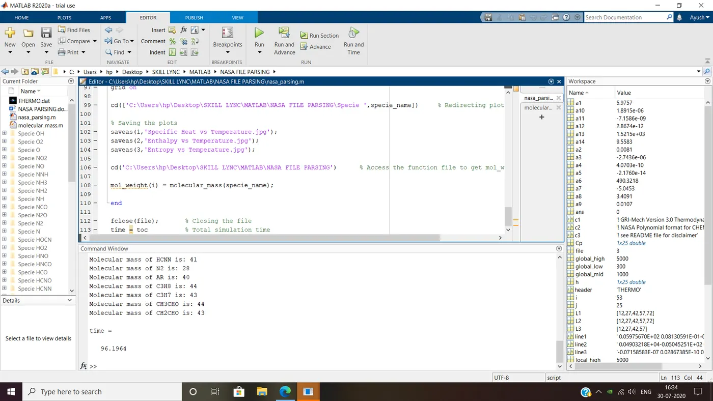
Folders for species:

Molecular weight of all species:

Plot: The Cp, h and S plots are plotted as shown.

O2 Plots:

N2 Plots:

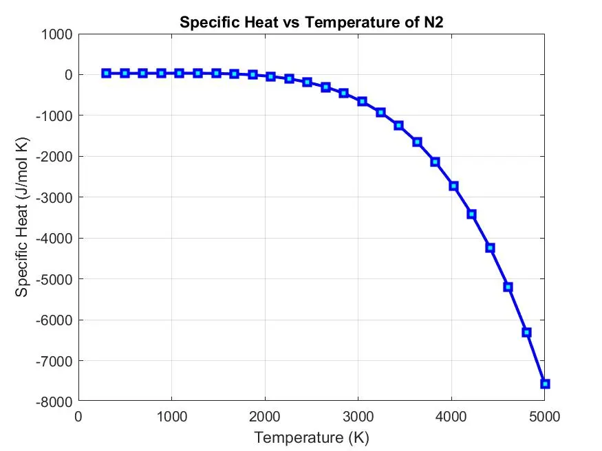
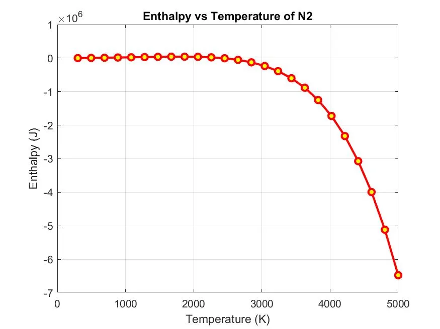
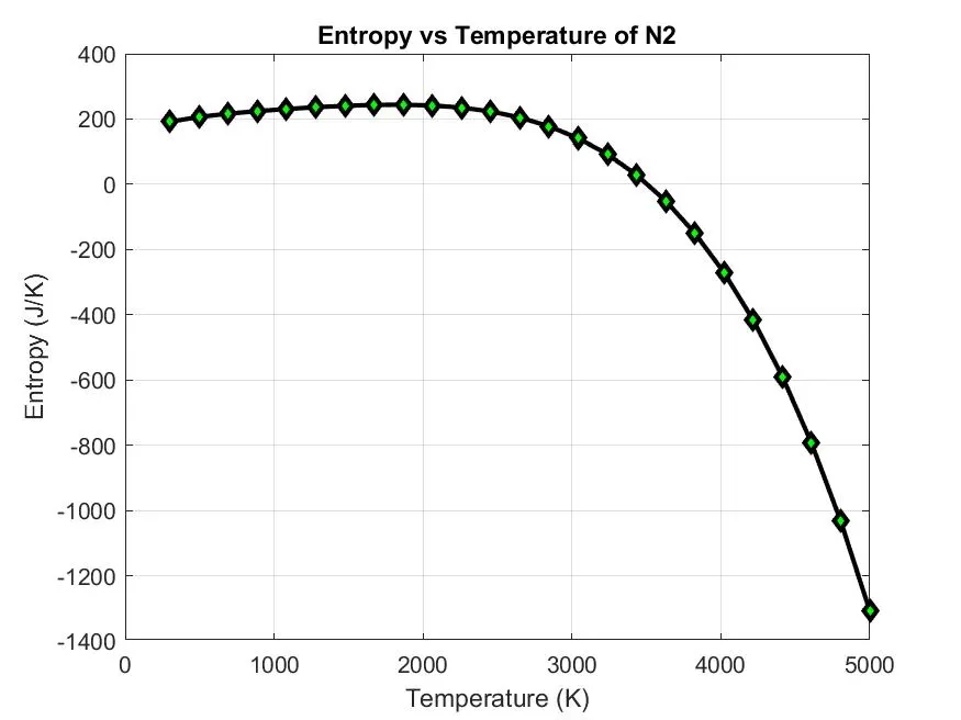
CO2 Plots:

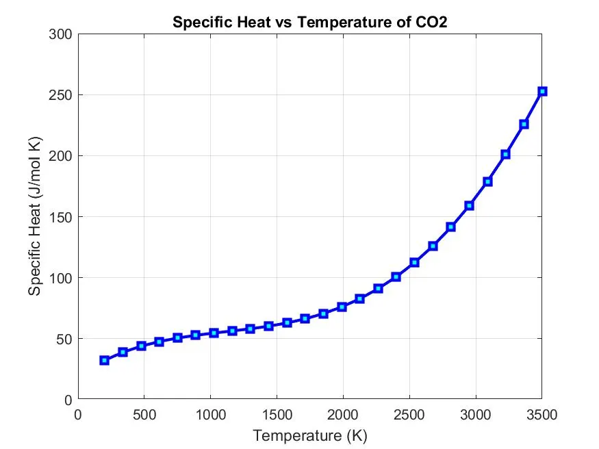
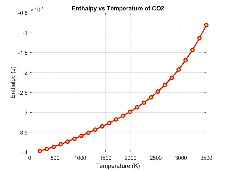
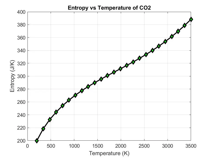
CONCLUSION: From the above results, we can see that the given problem statement is executed by calculating the thermodynamic properties and plotting the curves of all the species.

REFERENCES: THERMO.dat file