OTTO CYCLE SIMULATOR USING PYTHON

OBJECTIVE:

The primary objective of the project is to simulate the Otto cycle using Python and to create the PV diagram of the same. Also, to calculate the engine's thermal efficiency running in that cycle.

PROBLEM STATEMENT:

The engine's geometric dimensions are given along with the initial state parameters like temperature and pressure. With this details, the operating conditions of all the four states are to be calculated and in turn, engine's efficiency has also to be calculated. After this, the PV diagram of the cycle has to be plotted.

PROCEDURE:

Firstly, the dimensions of the engine are as follows.

1. Cylinder bore = 0.1 m
2. Stroke length = 0.1 m
3. Connecting rod length = 0.15 m
4. Compression ratio = 8
5. Specific heat ratio(Gamma) = 1.4

After this, the initial conditions are as follows.

1. Initial temperature = 500 K
2. Initial pressure = 101325 Pa

From the geometric dimensions, the swept volume and clearance volume are calculated. In this Otto cycle, there is 4 processes which are mentioned below.

1. Process 1 : Isentropic compression
2. Process 2 : Constant volume heat addition
3. Process 3 : Isentropic expansion
4. Process 4 : Constant volume heat rejection

Now, to simulate the four processes, we need to calculate the operating conditions at 4 state points. Once the 4 states are clearly defined, simulating the process is simple.

1. Process 1 : State 1 - 2
2. Process 2 : State 2 - 3
3. Process 3 : State 3 - 4
4. Process 4 : State 4 - 1

The parameters at different state points are calculated using laws for the respective processes. For isentropic compression and expansion, there is a law which is depicted below.

`pv^gamma = "constant"`

Also, all the processes are abide by this gas law:

`(pv)/t = "constant"`

With these equations, all the state point parameters are calculated. As we know, both isentropic processes are polynomial in nature, the curve representing those processes should have a non linear path. So, there is a need to calculate the points which represents the curve. So a combination of volume and pressure is calculated using a user defined function.

In that user defined function, using a range of crank angles from 180 degrees to 0 degrees, a list of volumes are calculated. After that, the pressure values corresponding to that volumes are calculated.

Program snippet:

# OTTO CYCLE SIMULATOR

# Importing essential libraries
import math
import matplotlib.pyplot as plt

# Function for calculating varying volumes
def engine_kinematics(bore, stroke, con_rod, cr, crank_start, crank_end):

	# Crank radius
	a = stroke/2
	# Ratio b/w connecting rod length and crank radius
	R = con_rod/a

	# Crank angles
	crank_angle = []
	cs = math.radians(crank_start)
	ce = math.radians(crank_end)

	num_angles = 100

	# Creating the list of crank angles
	for i in range(0,num_angles):
		temp = cs + i*(ce - cs)/(num_angles-1)
		crank_angle.append(temp)

	volume = []

	# Creating the list of volume of expansion
	for theta in crank_angle:

		term1 = 0.5*(cr-1)
		term2 = R + 1 - math.cos(theta)
		term3 = pow(pow(R,2) - pow(math.sin(theta), 2), 0.5)
		V = (1 + term1*(term2 - term3))*v_c
		volume.append(V)

	return volume

# Input parameters 
bore = 0.1
stroke = 0.1
con_rod = 0.15
cr = 8
gamma = 1.4

# Volume info
v_s = (math.pi/4)*pow(bore,2)*stroke  # Swept volume
v_c = v_s/(cr-1)  # Clearance volume

t3 = 2300 # in kelvin

# STATE POINT 1
t1 = 500 # in kelvin
p1 = 101325 # in pascal
v1 = v_s + v_c

# STATE POINT 2
v2 = v_c

# p1v1^gamma = p2v2^gamma
p2 = p1*pow(v1,gamma)/(pow(v2,gamma))

# p1v1/t1 = p2v2/t2  
constant = p1*v1/t1
t2 = p2*v2/constant

# Calculating volume change and pressure change during compression
v_compression = engine_kinematics(bore, stroke, con_rod, cr, 180, 0)

p_compression = []

for v in v_compression:
	p_compression.append(p1*pow(v1,gamma)/pow(v,gamma))


# STATE POINT 3
v3 = v2  # Constant volume heat addition

# p3v3/t3 = constant
p3 = constant*t3/v3

# STATE POINT 4
v4 = v1

# p3v3^gamma = p4v4^gamma
p4 = p3*pow(v3, gamma)/(pow(v4, gamma))
t4 = p4*v4/constant

# Calculating volume change and pressure change during expansion
v_expansion = engine_kinematics(bore, stroke, con_rod, cr, 0, 180)

p_expansion = []

for v in v_expansion:
	p_expansion.append(p3*pow(v3,gamma)/pow(v,gamma))


#Calculating the thermal efficiency of the engine
efficiency = (1 - ((t4-t1)/(t3-t2))) * 100
print('Thermal efficiency = ',efficiency, 'percent')

# Plotting the OTTO cycle's PV diagram
plt.title('PV diagram of OTTO cycle')
plt.plot(v_compression, p_compression,linewidth = 3)
plt.plot([v2,v3],[p2,p3],linewidth = 3)
plt.plot(v_expansion, p_expansion,linewidth = 3)
plt.plot([v4,v1],[p4,p1],linewidth = 3)
plt.xlabel('VOLUME')
plt.ylabel('PRESSURE')
plt.show()

After that, the thermal efficiency of the engine is calculated using the following equation:

`eta = 1- ((t_4-t_1)/(t_3-t_2))`

which can be described as,

Thermal efficiency of the engine = Work done / Heat input

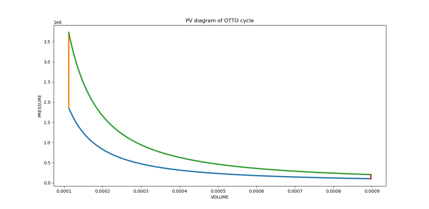
Then, plotting is done using the calculated values of pressure and volume which is called as the PV diagram of the Otto cycle.

RESULTS:

Output:

In the output, the thermal efficiency of the engine is printed as follows.

PV diagram of the Otto cycle:

CONCLUSION:

As we know, no engine or any machine is perfect and is not 100% efficient. There are a lot of losses involved. This engine working in the Otto cycle is no exception. It has considerable amount of heat losses and other losses too. That's why it cannot convert the heat energy into work completely making it only 56.4 % efficient. The PV diagram depicted is in good compliance with the curve generated by experimental values. The four processes are also depicted in a right manner which can be found in the nature of the curve. The losses can also be reduced by providing external cooling to the engine like fins or water(or oil) jackets. Also, it should be ensured that the proper combustion of the fuel takes place.